Tatooine¶

Modeling the One Star System¶

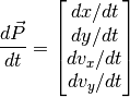
We first consider a planet orbiting a single star in a plane. The star is located at the origin, the position of the planet is (x, y), and the velocity of the planet has components (v_x, v_y). The state vector of the system is:

$\vec{P} = \begin{bmatrix} x \\ y \\ v_x \\ v_y \end{bmatrix}$

Given some initial state, we wish to calculate the future trajectory of the planet. To do this we need to derive formulas for the rate of change of each component of the state as a function of the current state.

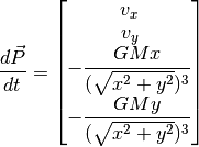
$\frac{d \vec{P}}{dt} = \begin{bmatrix} dx/dt \\ dy/dt \\ d v_x/dt \\ d v_y/dt \end{bmatrix}$

Newton’s “Law of Universal Gravitation” describes the force F acting on the planet in the direction of the star:

$|F| = \frac{GmM}{r^2}$

where

G is the gravitational constant
m is the mass of the planet
M is the mass of the sun
r is the distance of the planet from the star

Following Newton’s Second Law, F = ma, we divide the force F by the mass m of the planet to find the acceleration. The x component of the force is found by multiplying F by -x/r, while the y component is found by multiplying F by -y/r. Substituting r² = x² + y² then yields the differential equation governing the evolution of the system:

$\dfrac{d\vec{P}}{dt} = \begin{bmatrix} v_x \\ v_y \\ -\dfrac{GMx}{(\sqrt{x^2 + y^2})^3} \\ -\dfrac{GMy}{(\sqrt{x^2 + y^2})^3} \end{bmatrix}$

Numerical Solutions to Differential Equations¶

Euler’s Method¶

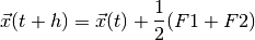
Euler’s method “solves” a differential equation by starting at an initial state and making repeated small changes to the state in the direction given by the derivative. If the initial state and differential equation are given by:

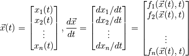
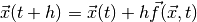
$\vec{x}(t) = \begin{bmatrix} x_1(t) \\ x_2(t) \\ \vdots \\ x_n(t) \end{bmatrix}, \dfrac{d\vec{x}}{dt} = \begin{bmatrix} d x_1/dt \\ d x_2/dt \\ \vdots \\ d x_n/dt \end{bmatrix} = \begin{bmatrix} f_1(\vec{x}(t), {t}) \\ f_2(\vec{x}(t), {t}) \\ \\ \vdots \\ f_n(\vec{x}(t), {t}) \end{bmatrix}$

Then by Euler’s method:

$\vec{x}(t+h) = \begin{bmatrix} x_1(t+h) \\ x_2(t+h) \\ \vdots \\ x_n(t+h)\end{bmatrix} \approx \begin{bmatrix} x_1(t) \\ x_2(t) \\ \vdots \\ x_n(t)\end{bmatrix} + h\begin{bmatrix} f_1(\vec{x}(t), {t}) \\ f_2(\vec{x}(t), {t}) \\ \\ \vdots \\[.05in] f_n(\vec{x}(t), {t}) \end{bmatrix}$

This can be summarized in vector form as:

$\vec{x}(t+h) = \vec{x}(t) + h \vec{f}(\vec{x}, t)$

The global error is O(h), so this is a first-order method.

Heun’s Method¶

A major problem with Euler’s method is that errors arise when the derivative changes. When the step size is large enough that the derivative changes significantly over a single step, these errors rapidly accumulate.

Heun’s method attempts to reduce these errors by taking into account the change in the derivative over each step. The core idea is that, instead of using the derivative at the start of a step to work out the direction of the step, we take the average derivative calculated at the start and end points of the step. Since we don’t know exactly where the end point is, Euler’s method is used to estimate the end point before calculating the average derivative.

This can be summarized in vector form as:

$\vec{x}(t+h) = \vec{x}(t) + \frac{1}{2}(F1 + F2)$

where

$\begin{cases} F_1 &= hf(\vec{x}, t) \\ F_2 &= hf(\vec{x} + F_1, t + h) \end{cases}$

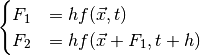
The global error is O(h²), so this is a second-order method.

Fourth-Order Runge-Kutta Method¶

The fourth-order Runge-Kutta method is a more sophisticated numerical differential equation solver. It can be summarized in vector form as:

$\vec{x}(t + h) = \vec{x}(t) + \frac{1}{6}(F_1 + 2F_2 + 2F_3 + F_4)$

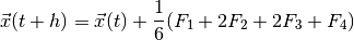
where

$\begin{cases} F_1 &= hf(\vec{x}, t) \\ F_2 &= hf(\vec{x} + \frac{1}{2}F_1, t + \frac{1}{2}h) \\ F_3 &= hf(\vec{x} + \frac{1}{2}F_2, t + \frac{1}{2}h) \\ F_4 &= hf(\vec{x} + F_3, t + h) \end{cases}$

This method is considerably more accurate than the previous two methods, with a global error of O(h⁴) (hence “fourth-order”).

Report Description¶

The report consists of the following exercises.

Part A: One Star System¶

Exercise 1. Solve the Equations of Motion for the One Star System

Develop a program using Heun’s method or the fourth-order Runge-Kutta method to simulate the dynamics of a planet orbiting a single star.

Exercise 2. Plot Trajectories for the One Star System

Generate and plot trajectories for the planet under a range of conditions to see what kinds of orbit exist. By “a range of conditions”, we mean that the initial position and velocity of the planet should be changed to observe the effect on the orbit.
Classify these orbits into a small number of types, and give an example of each.

Note

The simulation is more accurate with a smaller step-size h, but takes longer to run. Explain your reasoning in choosing a particular value for h, and how you know that it is small enough.

Tip

The Matplotlib function subplot can be used here to display many different planetary orbits on the same figure.

Part B: Two Star System¶

Exercise 3. Solve the Equations of Motion for the Two Star System

Modify the program to simulate the dynamics of a two star system.

Exercise 4. Plot Trajectories for the Two Star System

Generate and plot trajectories for the planet under a range of conditions for the two star system to see what kinds of orbit exist.
Classify these orbits into a small number of types, and give an example of each.

Exercise 5. Find the Closest Stable Orbit

Find an orbit as close as possible to the pair of stars that still seems stable. This can be done by moving the initial position of the planet closer to the suns and experimenting with different initial velocities to see what happens.

Exercise 6. Animate the Trajectory

Visualize the trajectory generated by adding animation to the simulation code.

Exercise 7. Explore Unequal Masses (Optional)

Explore some trajectories with unequal masses and see the effect on stability. The article on the website states that:

The larger star, Kepler-453A, is similar to our own Sun, containing 94% as much mass, while the smaller star, Kepler-453B, contains 20% as much mass ...

These masses might be an interesting place to start, scaled so that they sum to 1.

Hints and Suggestions for the Report¶

Write a calculate_path function to calculate the state of the planet for a given number of time steps.
Write a plot_path function which calls calculate_path to calculate the path, then plots the result.
Call plot_path with different arguments to generate different trajectories.

Incorporating Two Stars into the Simulation¶

The first simulation developed in class included a single star located at the origin. It was assumed that the mass of the star (M) was so much greater than that of the planet that the star could be considered as stationary. With two stars, this is no longer the case, and the changing positions of the stars needs to be taken into account.

We could compute the motion of the two stars by solving the differential equations that are Newton’s Laws. However, this is an unnecessary complication. Instead, we’ll treat the motion of the stars as a “solved” problem. The solution is that they both move in a circular orbit about their collective center of mass. This gives us a way to compute the positions of the stars at time t exactly.

Assume that the two stars are of mass M₁ and M₂, with M₁ + M₂ = 1.
Let the stars be one unit apart, with positions (x₁, y₁) and (x₂, y₂). Again for simplicity, let the center of mass be located at the origin. The distance of the first star from the origin is R₁ and the distance of the second star from the origin is R₂.
Assuming an angular velocity of 1, the positions of the stars are given by:

(x₁, y₁) = (R₁ cos t, R₁ sin t)

(x₂, y₂) = (-R₂ cos t, -R₂ sin t)
For simplicity, let M₁ = M₂ = 0.5. It follows that R₁ = R₂ = 0.5.

The Effect of Two Stars on the Planet¶

The main difference will be in the dP_dt function. This needs to be changed to take into account the positions and masses of the two stars. Forces simply add, so:

Modify the dP_dt function to include two forces, one towards each star.
Replace the x and y terms used to calculate the acceleration components ax and ay by x - x₁, y - y₁ for the first star and x - x₂, y - y₂ for the second star.

Incorporating Two Stars into the Animation¶

The main difference here is that the stars are now moving, rather than stationary.

The stars are now drawn objects that get updated during the animation.
These drawn objects need to be created at the same time as the planet and orbit objects that display the planet and its trajectory.
They need to be added to the fargs parameter list.
The data in these objects needs to be updated inside the animate function.
To be redrawn, these objects need to be returned from the animate functions.