Floating Point Numbers
Representing Numbers
The Base Ten System
The number system that we are used to dealing with in everyday life is based on powers of 10. In this system, an integer is represented as a sequence of digits from 0 to 9:

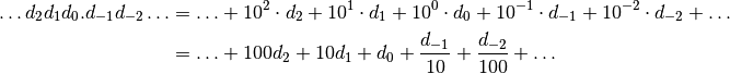
In the base 10 system, the value of a number is based on its position in the sequence. The right-most digit d0 indicates ones (or 100), the next digit d1 indicates tens (or 101), the next digit d2 indicates hundreds (or 102). So, the number d2 d1 d0 means 102 × d2 + 101 × d1 + 100 × d0. This system allows us to represent integers as large as we like by adding increasing powers of ten to the left.
We can extend this system to include numbers less than 1 by the addition of a decimal point:

The numbers to the right of the decimal point indicate negative powers of ten. The decimal part of this number therefore means 10-1 × d-1 + 10-2 × d-2 + ...
Putting the decimal part together with the integer part to the left of the decimal point, we have:
The dots  here indicate that we can make the number as large as we like by adding digits to the left, and as precise as we like by adding digits to the right.
Binary Numbers
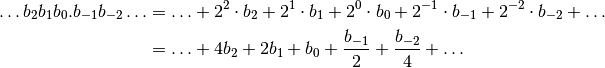
A binary number is based on powers of 2. As in the base 10 system, the value of a number is also based on its position in the sequence, and the powers used are powers of 2 rather than powers of 10. In the base 2 system, the only digits are 0 and 1. A number in this system is represented as a sequence of 1’s and 0’s:

The digits to the left of the point again represent the integer part of the number, and those to the right represent the fractional part.
An example of a binary integer is the number (1011)2. To convert this to base 10, we add up the powers of 2:

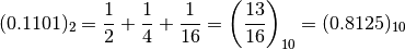
The fractional part to the right of the point is dealt with in the same way, but with negative powers of 2. For example:
Scientific Notation in Base Ten
Scientific notation allows us to represent very large and very small numbers without needing to write a decimal with a large number of zeros before or after the decimal point. Instead, we write a number as a decimal between 1 and 10, multiplied by a power of 10.
To convert a number to scientific notation, the decimal point is shifted to be immediately to the right of the leading digit. The number of spaces we need to move the decimal point tell us how large the power of 10 has to be.
- If the decimal point is moved to the left, we have a positive power of 10.
- If the decimal point is moved to the right, we have a negative power of 10.
Some examples are:
| 1234 | = | 1.234  103 103 |
decimal point moved 3 places to the left |
| 0.0000412 | = | 4.12 10-5 |
decimal point moved 5 places to the right |
| 456.789 | = | 4.56789 102 |
decimal point moved 2 places to the left |
Scientific Notation in the Binary (Base 2) System
Scientific notation works equally well in the binary (base 2) system. Just as in the base 10 system, we move the point to be immediately to the right of the leading digit, but in this case we multiply by a power of 2. Some examples are:
| 1011 | = | 1.011 23 |
point moved 3 places to the left |
| 0.00000110101 | = | 1.10101 2-6 |
point moved 6 places to the right |
| 11001.11 | = | 1.100111 24 |
point moved 4 places to the left |
The IEEE 754 Standard
The IEEE 754 standard defines a way to store a binary number on a computer. The standard is built on the following foundation:
- Every number is stored using the same, fixed number of binary digits, or bits (zeros and ones).
- The number of bits used depends on the computer and operating system used, but is usually either 32 or 64.
- Numbers are stored in binary scientific notation, as defined in the previous section.
- The power of 2 is referred to as the exponent, and the digits after the point as the mantissa.
- A fixed number of bits (E) are set aside to store the exponent, and a fixed number (M) to store the mantissa.
- A single bit - the sign bit - is used to indicate if the number stored is positive or negative. A sign bit of 0 represents a positive number, and a sign bit of 1 represents a negative number.
The Bias
The number stored in the bits set aside for the exponent represents a binary integer. As such, the minimum exponent value consists of all zeros, corresponding to the binary integer zero. This is not particularly useful, as it means that the smallest number we can store is 20 i.e. 1.
We would like however to be able to store both very large numbers (with a large positive exponent) and very small numbers (with a large negative exponent). To ovecome this problem, when a number in binary scientific notation is stored, a fixed integer (called the bias) is added to the actual exponent before it is stored.
For example, if we wanted to store the binary number 2-100, we would add the bias to -100 before it is stored in the exponent. The exponent stored would therefore be -100 + bias, rather than -100. When the stored exponent is converted back to the actual exponent, the bias therefore needs to be subtracted to get back to where we started.
Putting this together, we have a formula for converting the computer representation of a number back into an actual number in binary scientific notation:

The letter ‘s’ here denotes the value of the sign bit. Some examples are:
| Actual Number | Stored Number | |||
|---|---|---|---|---|
| Binary number | Scientific Notation | Sign | Exponent | Mantissa |
| 1011 | 1.011 × 23 | 0 | 3 + bias | 011000  000 000 |
| 0.00000110101 | 1.10101 × 2-6 | 0 | -6 + bias | 101010 000 |
| 11001.11 | 1.100111 × 24 | 0 | 4 + bias | 100111 000 |
Denormalized Numbers
A last problem to be solved is how to represent the number zero in this system. The assumption that a ‘1’ is always present before the mantissa bits doesn’t work, since the number zero doesn’t start with a ‘1’.
To solve this problem, a stored exponent of all zeros is treated differently from all other exponents. For the case when there is a stored exponent of all zeros:
- The assumption that the mantissa is preceded by a ‘1’ is dropped, and we assume that the mantissa is preceded by a ‘0’ instead.
- The actual exponent is taken to be 1 - bias.
Such a number is referred to as denormalized. This gives rise to a separate formula for converting the computer representation of a denormalized number back into an actual number in binary scientific notation:

Report Description
Part A: Finding the Floating Point Parameters
The first part of the report involves conducting experiments in Python to determine how many bits are used for the exponent (E) and mantissa (M), the value of the bias (B), and if denormalization is used. This is done by running experiments to find the machine epsilon, the smallest and the largest floating-point numbers.
Exercise 1. Machine Epsilon
- Write a function
find_epsilonthat finds the machine epsilon by determining the smallest floating point number larger than 1 that can be stored. - Call
find_epsilonto find this number. - Print both the number and the base 2 exponent for this number.
Exercise 2. Largest Floating Point
- Write a function
find_largestthat finds the largest floating point number that can be stored. - Call
find_largestto find this number. - Print both the number and the base 2 exponent for this number.
Exercise 3. Smallest Floating Point
- Write a function
find_smallestthat finds the smallest floating point number that can be stored. - Call
find_smallestto find this number. - Print both the number and the base 2 exponent for this number.
Exercise 4. Inferring Floating-Point Parameters
Fill in the rest of the table below.
| Number | Sign | Exponent | Mantissa | Value |
|---|---|---|---|---|
| Biggest float | ||||
| 1 + ϵ | 0 | B | 000 001 |
1 + 2-M |
| Smallest normalized | ||||
| “First” denormalized | 0 | 000...000 | 100 000 |
|
| Smallest float |
Then use the results of Exercises 1 - 3 to infer:
- The number of bits M reserved for the mantissa.
- The number of bits E reserved for the exponent.
- The bias B used for the exponent.
- Is denormalization used?
Note
Separate marks will be given for finding each of these numbers, for inferring the values of M, E, and B from them, and for determining if denormalization is used. The main thing is to justify the approach taken and reasoning used.
Part B: Extending the Taylor Series Approximation
The second part of the report involves the Taylor series approximation covered in class.
Exercise 5. Plot g(x) = log(1 + x)/x
- Plot the function g(x) = log(1 + x)/x when x is close to zero.
- Describe the main features of this graph and how they relate to the loss of precision when numbers of very different magnitudes are added or subtracted.
Exercise 6. Extend Taylor Series
- Extend the Taylor series approximation for this function that was begun in class by one more term.
- Plot the graph from Exercise 5 again along with the Taylor series approximation on the same graph.
Exercise 7. Approximation Error
- Find out how big x can be using this approximation while maintaining an error of less than or equal to 10-16.
Hints and Suggestions for the Report
Exercises 1, 2 and 3
The technique for finding each of these numbers is essentially the same: choose a power of 2, and increase (or decrease) it until the largest (or smallest) number that can be represented in Python is found. The algorithms to do this will follow that described in class for finding the machine epsilon.
Exercise 6
The Taylor series approximation to a function f(x), specialized to expansion at zero, is given by:

where ξ is some number between 0 and x. For the function g(x) = log(1 + x)/x, we can use this to derive a formula for f(x) = log(1 + x), then divide by x to get a formula for g(x).
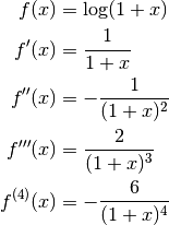
Evaluating f(x) and its derivatives at zero gives:

Hence:
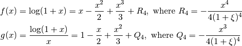
To finish Exercise 6, first derive one more term in this series (pun intended). Once this is done, plot both the approximation to g(x) (without the error term) and the original g(x) on the same graph.
Exercise 7
The term Q4 from Exercise 6 is a measure of the error associated with the approximation. If we know how this term is bounded for any value of ξ between 0 and x, then we know the maximum error using the approximation.
For 0 ≤ ξ ≤ x, the minimum value of 1 + ξ is when ξ = 0. Hence:
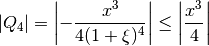
To find how big x can be while maintaining an approximation error of less than or equal to 10-16, we set Q4 ≤ 10-16 and solve for x. Completing Exercise 7 involves deriving one more term in the Taylor series expansion to find Q5, then solving again for x in the same way.