The Mayfly Model¶

The “Mayfly Model” is a simplified model of how the mayfly population of a given year depends on the population of the previous year. In this model the population in year t is given by a scaled measure x_t in the interval [0, 1].

The model assumes that in ideal conditions the number of surviving offspring per adult member of the population (including both males and females) is given by a parameter b. As the population rises, increased competition for resources, and population reduction by predators and disease, act to reduce the number of surviving offspring. Taking this effect into account, the population of the following year, x_t+1, is modeled by the recurrence relation x_t+1 = b x_t (1 – x_t).

The Butterfly Effect¶

For some dynamical systems, the initial state doesn’t have a lot of impact on the future development of the system. An example is the Mayfly model using certain ranges of values for the growth parameter b. In these cases, the dynamics of the system lead to the same long-term equilibrium behavior regardless of the initial population. The future is therefore relatively insensitive to the past, and the history of the system get “forgotten” over time.

The opposite of this is extreme sensitivity of the future to the past, or “sensitive dependence on initial conditions”. More formally, trajectories that start close together will separate exponentially. Over long enough periods of time this is enough to result in greatly differing outcomes regardless of how close two initial states are to each other. This kind of behavior is popularly known as the “Butterfly Effect”, the idea being that the flapping of the wings of a butterfly on one side of the world is enough to change the weather on the other side of the world some time later.

For certain values of b, the Mayfly model exhibits this kind of behavior. One of the tasks of this report is to explore this behavior, and find out the range of b values for which it occurs.

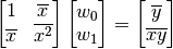
Simple Linear Regression¶

Given a set of data points {(x₁, y₁), (x₂, y₂), ..., (x_n, y_n) }, the parameters w₀ and w₁ of the straight line f(x) = w₀ + w₁ x that best fits the data are given by the solution to the matrix equation:

$\begin{bmatrix} 1 & \overline{x} \\ \overline{x} & \overline{x^2} \end{bmatrix} \begin{bmatrix} w_0 \\ w_1 \end{bmatrix} = \begin{bmatrix} \overline{y} \\ \overline{xy} \end{bmatrix}$

Report Description¶

Part A: The Mayfly Model¶

The goal of this report is to explore the Mayfly Model under a range of conditions. The primary question is: what kinds of behavior does the system x_t+1 = b x_t (1 – x_t) exhibit, and how do they depend on the parameter b? We are particularly interested in the different kinds of short-term (transient) and long-term (asymptotic) behavior that occur.

The report consists of the following exercises.

Exercise 1. Displaying the Transient Behavior

Run the mayfly model using several different values for b.
Plot the population against time over a sufficiently long period to allow the system to settle into a stable cycle (if possible).
Make some observations about your results.

Exercise 2. Displaying the Asymptotic Behavior

Generate a high-resolution picture of the values that the population converges to asymptotically for a large number of b values in the interval [0, 4].
Is this what you would expect?
Generate another picture zooming in on one area of the graph.
Make some observations about your results.
Do any kind of analysis you can to indicate what might be going on.

Part B: The Butterfly Effect¶

Exercise 3. Separation of Trajectories

We want to determine if the mayfly model exhibits a butterfly effect with b = 1.5, b = 4, and some other values of your choice.

See if trajectories that start very close together separate exponentially.
Graph the separation of nearby trajectories on a logarithmic scale against time using semilogy to plot log(s_t) against t.

Exercise 4. Linear Least Squares

Compute the growth rate of the separation during the time when it is growing exponentially. Use the “linear least squares” formula developed in class to compute the slope of the best-fit line on the logarithmic graph. The formula should be implemented from scratch in NumPy.
Graph both the separation of nearby trajectories and the “best fit” line to this separation on the same graph. Plotting them on the same graph is a way to confirm visually that the line has correctly fitted the data. If not, there is an error in the code somewhere.

Hints and Suggestions for the Report¶

Displaying the Asymptotic Behavior¶

The graph of the asymptotic behavior has a lot of detail that can easily be missed at low resolutions.

Use a large number of values for b.
Run the model for a sufficiently long period for the system to have converged to its asymptotic population values.
Use a small marker size.
Adjust the transparency of the points using the alpha value.
Use NumPy to vectorize your code and update the populations for all values of b together.

Initial Populations¶

We’re interested in the rate at which two initial populations m and n that start close together either grow further apart or closer together.

The initial populations should be very close, say only 10^-5 apart. The simplest way to do this is to choose one initial population m₀, then let the other population be n₀ = m₀ + ε where ε = 10^-5.
If things don’t seem to be working well with the initial population and separation you’ve chosen, try some others.
You may want to use a different initial population and separation for each b value. Experiment to find out what works best.

Updating the Populations¶

The populations m and n are both updated each year for a given value of b. At time t, they will have values m(t) and n(t).
The mayfly model x_t+1 = b x_t (1 – x_t) provides the formula to update the populations m and n each year.

Calculating the Separation¶

The “separation” between m(t) and n(t) is defined as s(t) = abs(m(t) - n(t)).

Plotting the Separation¶

Over a limited time period, s(t) should follow the formula for exponential separation given by s(t) = s(0) e^rt, where r is the rate at which the separation s(t) is growing.
The graph of log(s(t)) = log(s(0)) + rt should therefore be a straight line over some limited time period.

Linear Least Squares¶

When choosing data to apply the linear least squares formula to, make sure that the data is actually a straight line over this period.
When you use the linear least squares formula to find the coefficients w₀ and w₁, this needs to be done using y = log(s(t)) and x = t. This is because we are trying to fit a straight line to the log of the separation s(t), not directly to the separation s(t).
If w₀ and w₁ are correct, then semilogy(t, exp(w₀ + w₁ t)) should show a straight line fit to the data over the time period you’ve chosen.

Hint

The matrix equation Aw = b can be solved using the NumPy function linalg.solve(A, b).
The NumPy function mean can be used to find the mean value of the elements of an array.

Growth Rate¶

Assuming that s(t) = s(0)e^rt, then log(s(t)) = log(s(0)) + rt = w₀ + w₁ t. So, the growth rate r is just the value w₁ found using linear least squares, without needing any other computation.