Newton in the Complex Plane¶

Finding the Roots of Equations¶

Given a function f(x), we often need to find the values of x for which f(x) = 0. These are the roots of the function. We examine and implement three methods for doing this below.

The Bisection Method¶

The bisection method for finding the root of a function is based on the “Intermediate Value Theorem” from calculus:

Suppose that f is continuous on the closed interval [a, b] and let N be any number between f(a) and f(b), where f(a) is not equal to f(b). Then there exists a number c in (a, b) such that f(c) = N.

A corollary of this theorem is as follows:

If f(a) and f(b) are of opposite sign, then zero is a number between f(a) and f(b). Hence, there must exist a number c in (a, b) such that f(c) = 0. This number c is a root of f, and the interval [a, b] is called a “bracket” of the root.

Given an initial bracket, the bisection method repeatedly halves the width of the bracket, while ensuring that the new bracket still contains a root.

Choose a “bracket” [a, b] of the root with sign(f(a)) and sign(f(b)) opposite.
Evaluate f at the midpoint c.
“Replace” either a or b by c, to keep f(a) and f(b) of opposite sign.
Repeat until the bracket width (b - a) is within the desired tolerance.

Functional Iteration¶

Start with some guess x₀ at the solution (the root of f).
Generate a sequence of hopefully improving approximations x₁, x₂, ... by x_i+1 = f(x_i) + x.

Newton’s Method¶

For the two previous methods, all we had to use were the values of the function at a point. Newton’s Method also makes use of the function derivative. We would hope that having more information about a function will result in faster convergence to a root, and will see that this is in fact the case.

Newton’s Method proceeds as follows:

Assume that f is differentiable and values are available for both f and the derivative f’.
Start with an initial estimate x₀ of the root.
Find the tangent to f(x) at the current estimate, x₀.
Let x₁ be the intersection of the tangent with the x-axis. This is found using:

x_i+1 = x_i - f(x_i)/f’(x_i).
Continue to generate a sequence of (hopefully) better estimates to the root, x₁, x₂, ...

Complex Numbers¶

Complex numbers can be considered as pairs of real numbers, z = (x, y), with the following rules of arithmetic defined on them:

(x₁, y₁) + (x₂, y₂) = (x₁ + x₂, y₁ + y₂)
(x₁, y₁) - (x₂, y₂) = (x₁ - x₂, y₁ - y₂)
(x₁, y₁) * (x₂, y₂) = (x₁ x₂ - y₁ y₂, x₁ y₂ + x₂ y₁)

As with the real numbers, division is defined as “multiplication by the reciprocal”. The reciprocal of a complex number is the number which, when multiplied by it, gives the multiplicative identity 1. For a complex number (x, y), the reciprocal can be be shown to be:

$\left(\frac{x}{x^2 + y^2}, \frac{-y}{x^2 + y^2}\right)$

This gives us a system of arithmetic for complex numbers similar to that for real numbers. This system allows polynomial functions of complex variables to be defined, and the derivatives of such functions to be found. Newton’s Method can therefore be used to find the complex roots of a polynomial, in the same way that it can be used to find the real ones.

Polar Representation of Complex Numbers¶

We can represent a complex number (x, y) as a point in the “complex plane” in polar form (r, θ). The distance of a point from the origin is given by r, while the angle between the positive real axis and a line connecting the origin to the point is given by θ.

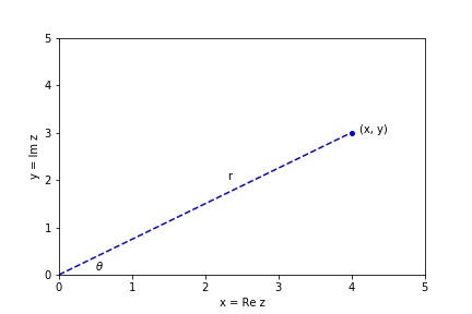
Conversion between the two coordinates systems is performed using:

(x, y) = (r cos θ, r sin θ)
(r, θ) = (sqrt(x² + y²), arctan(y/x))

Multiplication of two numbers in polar form is particularly simple. In polar form, the product of two complex numbers (r₁, θ₁) and (r₂, θ₂) is given by:

(r₁, θ₁) * (r₂, θ₂) = (r₁ * r₂, θ₁ + θ₂).

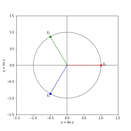
The Cube Roots of Unity¶

The cube roots of unity are the numbers z such that z³ = 1. In polar form, z = (r, θ), so z³ = (r³, 3 θ). Solving for r and θ gives r = 1 and θ = 0, 2π/3 and 4π/3.

These three roots ξ₀, ξ₁ and ξ₂ are shown below, equally spaced on the unit circle in the complex plane.

Report Description¶

The topic of this report is an exploration of how points in the complex plane converge to the “cube roots of unity” under Newton’s method. The report consists of the following exercises.

Exercise 1. Apply Newton’s Method in the Complex Plane

Choose a rectangular region of the complex plane that includes the origin. Use Newton’s method applied to the equation f(z) = z³ - 1 to find which of the three “cube roots of unity” different points in this region converge to.

Exercise 2. Display the Basins of Attraction

Generate a high-resolution image that colors the points in the region from Exercise 1 according to which of the three roots they converge to. You can use red, green, and blue, or some other set of three colors of your choice.
Make some observations about your results.

Exercise 3. Zoom in on the Complex Plane

Make an additional zoomed in picture of some “interesting” region.
Make some observations about your results.

Exercise 4. Display the Number of Iterations

Make a picture that uses the brightness of the color to represent the number of iterations needed by Newton’s method to converge to a root.
Make some observations about your results.

Hints and Suggestions for the Report¶

Generating the Image¶

Use meshgrid to generate an array of points in the complex plane, then apply Newton’s method to the entire array.
Find the root that each point converges to by checking if each point ends up closer to the root than some given tolerance.
Set each component of the color separately, or use NumPy indexing with boolean arrays to set the entire color according to the root.
Increase the number of points used to obtain an image of high resolution.
Use enough iterations of Newton’s method to minimize any black areas in the image. These correspond to points that have not converged to any of the three roots.
Images can be displayed using imshow.

Making a Zoomed in Picture of Some “Interesting” Region¶

The arguments to linspace can be modified to select a particular region of the complex plane.
How you define “interesting” is up to you, within limits. For example, a picture of a solid red square does not count as interesting in this context.

Displaying the Number of Iterations¶

The “number of iterations” refers to how many steps Newton’s method requires for a given point in the complex plane to converge to a root.
The code you develop for Exercise 1 can already detect if a point has converged to a given root. However, this is only run once, after Newton’s method has finished. To find the number of iterations needed, modify this code to test for convergence to a root after each iteration of Newton’s method.
The number of iterations needed will be an integer less than or equal to the maximum number of iterations. To be encoded as a brightness, this will need to be scaled to a float in the interval [0, 1] and applied to the appropriate color components.
The easiest way to scale the number of iterations back to [0, 1] is to divide by the total number of iterations. However, any function that maps from [0, num_iterations] to [0, 1] can be used. Interesting visual effects can be produced by choosing different functions to do this.