The Generation and Use of Random Numbers¶

Linear Congruential Generators¶

A linear congruential generator generates a sequence of numbers in the interval [0, 1) using the following algorithm:

Pick a multiplier a and modulus m, both large integers.
Pick a starting integer x₀ (your choice) in {1, 2, ... , m - 1}.
Generate a sequence of real numbers u_i by:

$x_{i} &= a * x_{i-1} \mod m \\ u_{i} &= x_{i}/m$

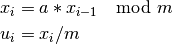
Report Description¶

Exercise 1. Linear Congruential Generators

Write a function rng that implements a linear congruential generator with the values a = 427419669081, m = 999999999989.
Write a function randu that implements a linear congruential generator with the values a = 2 ¹⁶ + 3, m = 2 ³¹.
Test the linear congruential generators in your rng and randu functions, and the generator in numpy.random.rand for (i) uniformity, and (ii) lack of (coarse-scale) successive pair correlation.

Exercise 2. Estimate the Value of Pi

Use Monte Carlo Integration to estimate the area of a circle of radius 1 (which gives us an estimate of the value of pi).

Exercise 3. Bernoulli Random Variables

In a game of tennis, Serena has a 60% probability to win any given point against Venus. Games are won by the first player to get to 4 points.

What do you expect Serena’s probability of winning a game to be - less than, greater than, or equal to 60%?
Simulate the results of a large number of games.
Plot a histogram of the number of points scored by Serena in each game.
Numerically estimate the probability of Serena winning a game. Is this the result you expected?

Exercise 4. Sums of Random Variables

Produce a histogram of the sums of pairs of uniformly distributed random numbers produced by numpy.random.rand.
Produce histograms for the sums of M-tuples of uniform random numbers for values of M greater than 2.
See if it is possible to shift and stretch the sums of M-tuples so that their distribution converges to something as M increases without bounds.

Exercise 5: The Exponential Distribution

The exponential distribution is used to model the time interval between events that occur randomly and independently in time. The probability density function for this distribution is:

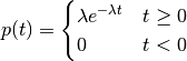
$p(t) = \begin{cases} \lambda e^{-\lambda t} & t \geq 0 \\ 0 & t < 0 \end{cases}$

where λ > 0 is a parameter governing the mean time interval between events.

An example of an exponential distribution is radioactive decay, such as when Carbon-14 atoms decay to Nitrogen-14. In this case, the exponential distribution is a probability density function describing the time for an atom to decay. Since the mean time for an atom to decay is 8267 years, λ is given by 1/8267.

Using λ = 1/8267, construct a function g(u) so that t = g(u) has the pdf p(t) given above.
Confirm that the histogram of a large number of random numbers generated using t = g(u) does actually match the probability density function p(t).
Plot the sums of M-tuples of exponentially distributed random numbers to see if these sums also converge to some limiting distribution. There is no need to do any kind of detailed analysis here.

Exercise 6. To Switch or Not to Switch

The math department is having a competition. There are three sealed boxes. Two of the boxes are empty, and the third box contains a bonus quiz card for MTH 337 (we don’t have a lot of money for prizes). You’re not told which box contains the card, but the instructor knows which one does.

You choose a box. The instructor then opens one other box, and shows you that it’s empty. You are then offered a choice. You can stick with the box you initially chose, or you can switch to the remaining other box. What should you do?

Describe the choice you would make, and why.
Using a large number of trials, simulate the result of sticking with your original choice, and of switching to the other box.
How often would you win (on average) using each of the two strategies?

Exercise 7. Stock Market Model

The simple stock price model defined in class is:

s(t + 1) = (1 + μ + σ ε) s(t)

where:

s(t) is the stock price at time t.

μ is an underlying rate of growth per step.

ε is a “stochastic” or random term with a normal distribution.

σ is the volatility, the amplitude of the stochastic term.

Implement this model using a value for μ of 0.0 and σ of 0.05 to find out what happens to an initial investment of 1 unit of money over 365 time steps.
Plot the changing price of several stocks over this period.
Plot a histogram of final stock prices after 365 steps using a large number of trials.
Estimate the “expected value” (average over all trials) of the investment after 1 year.
Calculate the likelihood of losing money. This is the proportion of trials where s(365) ends up less than 1.
Calculate the “most likely” value of the investment after 1 year, using an appropriate definition of “most likely”.
Draw some conclusion about investing, or on the value of money.
Run another simulation using a more modest value for σ of 1%. Describe how changing σ affects the final distribution i.e. the histogram of final prices.

Hints and Suggestions for the Report¶

Linear Congruential Generators¶

Testing for uniformity is done by plotting a histogram showing the distribution of the points in the interval [0, 1].
- Use enough bins for the histogram to provide a clear idea of the shape of the distribution.
- Use enough points that every bin in the histogram contains a large number - the more points the better.
Testing for pairwise correlation is done by plotting successive pairs (u_i, u_i+1) as points in the plane.
- Use lots of points, to see how effectively the points fill the unit square.
- Use a small marker size, so that markers do not overlap.

Estimating Pi¶

The circle is contained in a bounding box [-1, 1] $\times$ [-1, 1] in the xy-plane.
Use rand to generate a large number of points, then scale the output of this function so that points (x, y) are uniform inside this box. An appropriate transformation is u → 2u - 1.
Use hypot to find the value of r corresponding to each (x, y) pair.
A point (x, y) is inside the circle if r < 1.

Bernoulli Random Variables¶

Treat each point as a Bernoulli random number with p = 0.60.
Numerically estimate Serena’s probability of winning a game by running a large number of games, each of which consists of 7 points. We want the proportion of games where Serena scores 4 or more points.
The most compact way to do this is to start with a 2D NumPy array of shape (7, ngames) generated using rand.
A combination of operations applied directly to this array (to turn a uniform random number into a Bernoulli random number, for example), and an axis-dependent operation (for counting the points per game), will allow the result to be found without using any “for” loops.

Generating Histograms of M-Tuple Sums¶

Use rand to create a 2D NumPy array of shape (M, npts).
Sum all the M-tuples using sum as an axis-dependent operation i.e. by specifying which axis to sum over.

Finding the “Right” Scaling¶

The “right” scaling is a function of M. When divided by this scaling, the histograms produced for different values of M should converge to the same distribution as M increases without bound.
For each histogram generated for a different value of M, first subtract the mean (M/2) to shift the histogram so that it is centered on zero.
Use the normed=True keyword argument to hist to turn the histogram into a probability distribution.
Consider using the histtype='step' keyword argument when plotting multiple histograms on the same axes. This just plots the outline of a histogram, so it may be easier to see when convergence is happening.

The Exponential Distribution¶

Construct a function g(u) so that t = g(u) has the exponential pdf p(t). Remember from class that the steps to construct this function are:
1. Let $u = \int p(t) dt$
2. Plug in your probability density function p(t), and integrate to find u as a function of t.
3. Solve for t as a function of u, given by t = g(u).
Sum M-tuples of large numbers of samples drawn from p(t) using t = g(u). Remember that using a NumPy 2D array of shape (M, npts) will allow this kind of summing to be performed very efficiently.

To Switch or Not to Switch¶

Use an integer from the set {1, 2, 3} to represent each box.
Use numpy.random.randint to randomly select winning boxes for a large number of trials.
Construct an array of box choices made using each of the two strategies.
Compare the winning box to your choice in both cases using ==, then use np.sum to sum the number of wins.

Plotting the Changing Stock Prices¶

The random ε term needs to be calculated separately for every step.
A “for” loop will be needed since the stock price each day is calculated from the previous day.
Prices {s(0), s(1), ..., s(365)} should be saved either to a list or into an array.
Plot enough stock prices to see how much variation there is in the different stock trajectories.
Note that plot can be passed a 2D array to plot. When this is done, each column is plotted as a separate line.

Plotting the Histogram of Final Prices¶

A large number of stock prices need to be tracked to get a good idea of the final distribution.
A 1D array can be used to store the current prices of the different stocks. These prices can all be updated together each day inside the “for” loop.
After the “for” loop is complete, this 1D array will contain the final price for every stock.

Analyzing the Distribution of Final Prices¶

The array of final stock prices can be used to find both the expected value, the likelihood of losing money, and the “most likely” value of the investment after 1 year.