The Generation and Use of Random Numbers¶

Report Description¶

Exercise 1.

Write a function rng that implements a linear congruential generator with the values a = 427419669081, m = 999999999989.
Write a function randu that implements a linear congruential generator with the values a = 2 ¹⁶ + 3, m = 2 ³¹.
Test the linear congruential generators in your rng and randu functions, and the generator in random.rand for (i) uniformity, and (ii) lack of (coarse-scale) successive pair correlation.

Note

Testing for uniformity is done by plotting a histogram showing the distribution of the points in the interval [0, 1].
Testing for pairwise correlation is done by plotting successive pairs $(x_i, x_{i+1})$ as points in the plane.

Tip

Use enough bins for the histogram to provide a clear idea of the shape of the distribution.
Use enough points that every bin in the histogram contains a large number - the more points the better.

Exercise 2. Use Monte Carlo integration to find the mean of the function mysteryf in the mystery module by random sampling over the interval [0, 5].

Mystery module

Note

Use an appropriately large number of samples generated using random.rand.
Scale the points returned by random.rand so they are uniform in the interval [0, 5], not [0, 1].

Tip

The formula for the mean of a function is:

$\overline{f} = \dfrac{1}{n} \sum_{i=1}^{n} f(x_i)$

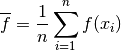
This can be calculated using NumPy array operations and mean without needing “for” loops.
The mean can be estimated a few times to get an idea of how accurate the estimate is.

Exercise 3. Use Monte Carlo integration to estimate the area of the “flower” whose boundary has the equation 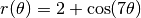$r(\theta) = 2 + \cos(7\theta)$ in polar coordinates.

Tip

The “flower” is contained in a bounding box [-3, 3] $\times$ [-3, 3] in the xy-plane. Use random.rand to generate a large number of points, then scale the output of this function so that points (x, y) are uniform inside this box. An appropriate transformation is $u \rightarrow 6u - 3$ .
Use arctan2 to find the value of $\theta$ corresponding to a given (x, y) pair.
Use the function definition for $r(\theta)$ to work out if a point is inside the curve (if 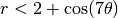$r < 2 + \cos(7\theta)$ , then the point is inside the curve).

Exercise 4. Numerically estimate the probability of getting 29 hits in 100 swings in a baseball game if the probability of getting a hit on any one swing is 0.29 (and is independent of other swings).

Tip

Treat each swing as a Bernoulli random number with p = 0.29.
Numerically estimate the probability by running a large number of trials, each of which consists of 100 swings. We want the proportion of trials with exactly 29 hits.
The most compact way to do this is to start with a 2D NumPy array of shape (100, ntrials) generated using random.rand.
A combination of operations applied directly to this array (to turn a uniform random number into a Bernoulli random number, for example), and an axis-dependent operation (for counting the hits per trial), will allow the result to be found without using any “for” loops.

Exercise 5.

Produce a histogram of the sums of pairs of uniformly distributed random numbers produced by random.rand.
Produce histograms for the sums of M-tuples of uniform random numbers for values of M greater than 2.

Tip

Use random.rand to create a 2D NumPy array of shape (M, npts).
Sum all the M-tuples using sum as an axis-dependent operation i.e. by specifying which axis to sum over.

See if it is possible to shift and stretch the sums of M-tuples so that their distribution converges to something as M increases without bounds.

Tip

The “right” scaling is a function of M. When divided by this scaling, the histograms produced for different values of M should converge to the same distribution as M increases without bound.
For each histogram generated for a different value of M, first subtract the mean (M/2) to shift the histogram so that it is centered on zero.
Use the normed=True keyword argument to hist to turn the histogram into a probability distribution.
Consider using the histtype=’step’ keyword argument when plotting multiple histograms on the same axes. This just plots the outline of a histogram, so it may be easier to see when convergence is happening.

Plot the sums of M-tuples of non-uniform random numbers to see if these sums also converge to some limiting distribution. There is no need to do any kind of detailed analysis here.

Tip

Choose some other non-uniform probability density function, p(v). It can be any function you like, as long as both:
- $p(v) \geq 0$ for all v
- $\int\limits_{-\infty}^{\infty} p(v) dv = 1$ .
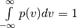Construct a function g(u) so that v = g(u) has the pdf p(v). Remember from class that the steps to construct this function are:
1. Let $u = \int p(v) dv$
2. Plug in your probability density function p(v), and integrate to find u as a function of v.
3. Solve for v as a function of u, given by v = g(u).
Sum M-tuples of large numbers of samples drawn from p(v) using v = g(u). Remember that using a NumPy 2D array of shape (M, npts) will allow this kind of summing to be performed very compactly.

Exercise 6.

Implement the simple stock price model defined in class using a value for $\mu$ of 0.0 and $\sigma$ of 0.05 to find out what happens to an initial investment of 1 unit of money over 365 time steps. The model is:

$s(t + 1) = (1 + \mu + \sigma \varepsilon) s(t)$

Note

$s(t)$ is the stock price at time t.
$\mu$ is an underlying rate of growth per step.
$\varepsilon$ is a “stochastic” or random term with a normal distribution.
$\sigma$ is the volatility, the amplitude of the stochastic term.

Important

The random $\varepsilon$ term needs to be calculated separately for every step.

Tip

A “for” loop will be needed since the stock price each day is calculated from the previous day.
Prices $\{s(0), s(1), ..., s(365)\}$ should be saved either to a list or into an array.

Plot the changing price of several stocks over this period.

Tip

Plot enough stock prices to see how much variation there is in the different stock trajectories.
Note that plot can be passed a 2D array to plot. When this is done, each column is plotted as a separate line.

Plot a histogram of final stock prices after 365 steps using a large number of trials.

Tip

A large number of stock prices need to be tracked to get a good idea of the final distribution.
A 1D array can be used to store the current prices of the different stocks. These prices can all be updated together each day inside the “for” loop.
After the “for” loop is complete, this 1D array will contain the final price for every stock.

Estimate the “expected value” (average over all trials) of the investment after 1 year.
Calculate the likelihood of losing money. This is the proportion of trials where s(365) ends up less than 1.
Calculate the “most likely” value of the investment after 1 year, using an appropriate definition of “most likely”.

Tip

The array of final stock prices can be used to find both the expected value, the likelihood of losing money, and the “most likely” value of the investment after 1 year.

Draw some conclusion about investing, or on the value of money.
Run another simulation using a more modest value for $\sigma$ of 1%. Describe how changing $\sigma$ affects the final distribution i.e. the histogram of final prices.