Cellular Automata
A cellular automaton is a self-contained stylized universe in which space is divided into a regular grid of cells. Each cell has a state and a set of close neighbors. Time advances in discrete steps. At each step the state of every cell is updated according to a transition rule based only on the states of the cell and its neighbors.
The transition rule can be thought of as describing the “laws of physics” for the system that the cellular automaton models. These laws are local (dependent only on the state of the cell and its neighbors) and uniform (the same for every cell).
The cellular automaton described in class has:
- A one-dimensional grid. Each cell has just two neighbors, one on either side.
- Four possible cell states (0, 1, 2, 3), each of which is represented by a different color.
- Periodic edge conditions - the rightmost and leftmost cells are neighbors.
- A transition rule where the state of each cell is updated based on the sum of the current cell state and those of its neighbors.
Report Description
The report involves implementing this one-dimensional cellular automaton and exploring the range of behaviors that different transition rules can give rise to.
- Implement the cellular automaton using NumPy arrays and array operations.
Note
Four NumPy arrays will be needed for the implementation.
- Cell states
- This is a 2D integer array where each row represents one generation of cells.
- Start with an empty NumPy array of the shape needed.
- The number of columns is the number of cells.
- The number of rows is the number of generations.
- Randomly initialize the first row using random.randint.
- Generate each row from the previous row using the transition rule.
- The “=” operator can be used to assign values to cells.
- Transition rule
- This is a 1D integer array with 10 elements in the range [0, 3].
- Colors
- This is a 2D float array of shape(4, 3).
- Each row contains a three element RGB color corresponding to a cell state.
- Image
- This is a 3D float array created by mapping cell states to colors.
- Display this image using imshow.
- Make your own choices for the colors used to indicate the state of each cell.
Tip
NumPy integer array indexing can be used to both:
- convert the array of cell states to an image array, and;
- generate each row from the previous row using the transition rule.
- Experiment with lots of different transition rules, then classify them into a small number of different types based on the long-term behavior of the system. Run the cellular automaton with each transition rule for as many generations as you feel are necessary to see the long-term behavior.
Tip
random.randint can also be used to generate random transition rules. This may be a more effective way to explore a large number of possible rules than creating rules by hand.
- If possible, identify some features of the transition rules that give rise to the different kinds of behavior.
Note
Show several examples for each class of behavior. The Matplotlib function subplot may be useful here for displaying lots of images in a single figure.
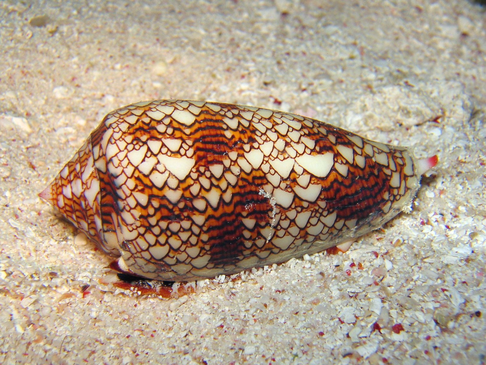
- If you have time, try to find a rule that will generate a pattern similar to the Textile Cone shell shown below.