Mauna Loa CO2 Levels¶

Report Description¶

Exercise 1: Load and Plot the Data.

Download the Mauna Load CO₂ data from the “National Oceanic and Atmospheric Administration” website and save it to a local file named “co2_mm_mlo.txt”.
Load the data into a NumPy array using NumPy’s loadtxt function and plot the monthly CO₂ levels against time in years.
Make some observations about your results.

Exercise 2: Simple Linear Regression.

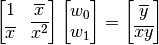
Given a set of data points $\{(x_1, y_1), (x_2, y_2) \ldots, (x_n, y_n)\}$ , the parameters $w_0$ and $w_1$ of the straight line 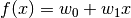$f(x) = w_0 + w_1 x$ that best fits the data are given by the solution to the matrix equation:

$\begin{bmatrix} 1 & \overline{x} \\ \overline{x} & \overline{x^2} \end{bmatrix} \begin{bmatrix} w_0 \\ w_1 \end{bmatrix} = \begin{bmatrix} \overline{y} \\ \overline{xy} \end{bmatrix}$

Find the “best fit” of a straight line to the data using the solutions $w_0$ and $w_1$ as the parameters for the straight line. Plot this straight line along with the original data on the same graph.
Predict CO₂ levels in the years 2050 and 2100 on the basis of this model.
Plot the residual difference against time between the original data and this straight line.
Make some observations about your results.

Hint

The matrix equation Aw = b can be solved using the NumPy function linalg.solve(A, b).
The NumPy function mean can be used to find the mean value of the elements of an array.

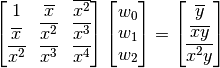
Exercise 3: Fitting a Quadratic Function.

The parameters $w_0$ , $w_1$ and $w_2$ of the quadratic function 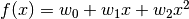$f(x) = w_0 + w_1 x + w_2 x^2$ that best fits the data are given by the solution to the matrix equation:

$\begin{bmatrix} 1 & \overline{x} & \overline{x^2} \\ \overline{x} & \overline{x^2} & \overline{x^3} \\ \overline{x^2} & \overline{x^3} & \overline{x^4} \end{bmatrix} \begin{bmatrix} w_0 \\ w_1 \\ w_2 \end{bmatrix} = \begin{bmatrix} \overline{y} \\ \overline{xy} \\ \overline{x^2y} \end{bmatrix}$

Find the “best fit” of a quadratic function to the data using the solutions $w_0$ , $w_1$ and $w_2$ as the parameters for the function. Plot this curve along with the original data on the same graph.
Predict CO₂ levels in the years 2050 and 2100 on the basis of this model.
Plot the residual difference against time between the original data and this curve.
Make some observations about your results.

Tip

The linear and quadratic models for the CO₂ data should actually fit the data! Plotting them on the same graph as the original data is a way to confirm this visually. If not, there is an error in the code somewhere.

Exercise 4: Seasonal Variation.

Plot the residual difference against month of the quadratic residuals.
Plot the mean monthly residual difference of the quadratic residuals on the same graph.
Plot the remaining residuals after the mean monthly residuals have also been removed.
Make some observations about your results.

Note

For each of these exercises, say how you have used NumPy arrays, indexing and slicing, and array operations to perform these tasks.