The Magnetic Pendulum¶

A pendulum is viewed from above, suspended from a pivot at the origin. Magnets at positions $(x_i, y_i)$ attract another magnet at the end of the pendulum. The position of the pendulum magnet is $(x, y)$ , and the state vector of the system is:

$\vec{P} = \begin{bmatrix} x \\ y \\ v_x \\ v_y \end{bmatrix}$

Three kinds of force act on the pendulum magnet: gravitational, frictional, and magnetic.

Gravity¶

Under the assumption that the horizontal displacement of the pendulum is small relative to the length of the pendulum, the restoring force of gravity towards the origin is directly proportional to distance from the origin. The parameters governing the acceleration due to gravity can be combined into a single coefficient C.

Friction¶

For low velocities we make the simplifying assumption that frictional forces act opposite to and directly proportional to velocity. The parameters governing friction can be combined into a single coefficient R.

Magnetism¶

The plane and pendulum magnets are modelled as magnetic dipoles with magnetic moments $\mathbf{m}$ for the pendulum and $\mathbf{m}_i$ for plane magnet i. We make the simplifying assumption that the pendulum is sufficiently long that the height of the magnet over the plane is a constant d and that the dipoles are vertically aligned with each other.

There is a standard formula that we can use for the force between two magnetic dipoles separated by a distance vector $\mathbf{r}$ . To make use of this formula, we first express $\mathbf{m}$ , $\mathbf{m}_i$ and $\mathbf{r}$ in vector component form where $\mathbf{i}$ , $\mathbf{j}$ and $\mathbf{k}$ are unit vectors in the directions of the x, y and z axes respectively.

$\mathbf{m} = m\mathbf{k}$ , where $m = |\mathbf{m}|$
$\mathbf{m}_i = m_i\mathbf{k}$ , where $m_i = |\mathbf{m}_i|$
$\mathbf{r}_i = (x - x_i)\mathbf{i} + (y - y_i)\mathbf{j} + d\mathbf{k}$ , so $r_i = |\mathbf{r}_i| = \sqrt{(x - x_i)^2 + (y - y_i)^2 + d^2}$

Plugging these component vectors into the standard formula yields the force $F_i$ exerted by the i th plane magnet on the pendulum magnet:

$\begin{eqnarray*} F_i(\mathbf{r}_i, \mathbf{m}_i, \mathbf{m}) & = & \frac{3\mu _0}{4\pi r_i^5}\left[(\mathbf{m}_i \cdot \mathbf{r}_i )\mathbf{m} + (\mathbf{m} \cdot \mathbf{r}_i )\mathbf{m}_i +(\mathbf{m}_i \cdot \mathbf{m}) \mathbf{r}_i - \frac{5(\mathbf{m}_i \cdot \mathbf{r}_i )(\mathbf{m} \cdot \mathbf{r}_i)}{r_i^2} \mathbf{r}_i\right] \\ & = & \frac{3\mu _0}{4\pi r_i^5}\left[m_i d m\mathbf{k} + m d m_i\mathbf{k} + m_i m ((x - x_i)\mathbf{i} + (y - y_i)\mathbf{j} + d\mathbf{k}) - 5 \frac{m_i m d^2}{r_i^2}((x - x_i)\mathbf{i} + (y - y_i)\mathbf{j} + d\mathbf{k})\right] \\ & = & \frac{3m_i m \mu _0}{4\pi r_i^5}\left[(x - x_i)\left(1 - \frac{5 d^2}{r_i^2}\right)\mathbf{i} + (y - y_i)\left(1 - \frac{5 d^2}{r_i^2}\right)\mathbf{j} + \left(3d - \frac{5 d^3}{r_i^2}\right) \mathbf{k}\right] \end{eqnarray*}$

The $\mathbf{i}$ and $\mathbf{j}$ components of the force $F_i$ can then be used to directly calculate the $x$ and $y$ components of the pendulum acceleration due to the plane magnets. For simplicity, the system is scaled so that the constant term $\frac{3m_i m \mu _0}{4\pi}$ = 1.

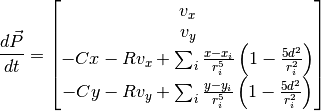
Adding up the different forces, the differential equation governing the evolution of the system is:

$\dfrac{d\vec{P}}{dt} = \begin{bmatrix} v_x \\ v_y \\ -Cx - R v_x + \sum_i \frac{x - x_i}{r_i^5}\left(1 - \frac{5 d^2}{r_i^2}\right) \\ -Cy - R v_y + \sum_i \frac{y - y_i}{r_i^5}\left(1 - \frac{5 d^2}{r_i^2}\right) \end{bmatrix}$

Report Description¶

The report consists of the following exercises.

Exercise 1. Simulate the dynamics of this system using the improved Euler method, and plot the path of the pendulum using several different initial states. Equally space three plane magnets on the unit circle, starting at (1, 0). Plot the position of the magnets as well when you plot the path of the pendulum.

Note

The simulation is more accurate with a smaller step-size h, but takes longer to run. Explain your reasoning in choosing a particular value for h, and how you know that it is small enough.

Exercise 2. Choose a value for d then repeat step 1 using the same initial state but with different values for C and R. Make some observations about the different kinds of path generated, and relate them to the physical system being modeled.

Tip

The Matplotlib function subplot can be used here to display several different pendulum paths on the same figure.

Exercise 3. Use the Matplotlib animation module to animate the path taken by the pendulum from one initial state.

Exercise 4. Divide the xy-plane into a grid of cells where each cell is considered a different starting point from rest for the pendulum. Assign a color to each magnet, then color each cell according to the magnet the pendulum finally ends up over.

Exercise 5. Repeat step 4 using different values for the frictional parameter R, and comment on the different kinds of image generated.

Important

Every report always needs an introductory section which describes the background to the report, the topic the report is exploring, and the tasks that the report is addressing.