Bouncing Ping-Pong Ball
When a ping-pong ball is dropped onto a hard surface, it bounces. It does not, however, bounce all the way back up. Such an event is referred to as an ‘inelastic collision’, meaning a collision in which some of the kinetic energy of the object is converted into other forms of energy, mostly heat and sound.
A simple mathematical model for an inelastic collision has the ball losing a fixed fraction of its energy on every bounce. In this model, we use the following notation:
 is the mass of the ping-pong ball.
 is the velocity after the ith bounce.
 is the time between bounce i and bounce i + 1.
 is the energy of the ball after the ith bounce. So,
  .
. is the acceleration due to gravity.
The equations of motion for the ball can be solved to give the height of the ball at time t after the ith bounce as:
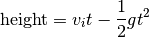
Setting this height equal to zero (for when the ball hits the surface again at the next bounce) and solving for  yields:

If we further assume that the fraction of energy retained after each bounce is a constant  then:
then:
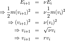
And so:
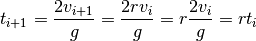
It follows that if this model is correct, then the time between bounces will be reduced by a fixed constant r with each bounce.
Report Description
The conjecture to be tested is that the behavior of a real bouncing ping-pong ball does in fact fit this model. This will be done by extracting the time between bounces from an audio file recording of a bouncing ping-pong ball and comparing them to the predictions of the model.
Exercise 1. Use scipy.io.wavfile.read to load the WAV file recording below of a bouncing ping-pong ball. Plot the sound amplitude against time, and make some observations about the resulting graph.
Exercise 2. The “spikes” in the WAV file correspond to the bounces of the ping-pong ball. Use this information to extract the time of each bounce from the WAV file. This can be done by either visually inspecting the plot of the sound amplitude, or (preferably) by writing code to extract the times for you. Plot the sound amplitude against time again, indicating on the same graph where the bounces occur.
Tip
- Storing the bounce times in a NumPy array will make analyzing the data easier for the remaining exercises.
- The Matplotlib function axvline can be used to add a vertical line to a graph.
Exercise 3. Calculate the least-squares straight line fit to the logarithm of the time intervals between bounces. Plot this line along with the original data to confirm that it is the correct fit. Use the results obtained to test the notion that a fixed fraction of the energy is lost on each bounce, and find an approximate value for this fraction.
Important
The linear regression algorithm developed for Report 3 must be used with the logarithm of the time interval between bounces, not directly with the time interval.
Note
The Matplotlib function semilogy will plot a function of the form  as the straight line
  . This can be used to plot the time between bounces.
Exercise 4. Plot a graph of the sound amplitude against time for a single bounce. Estimate by visual inspection of this graph the dominant frequency of the “ringing” of the ping pong ball after each impact.
Tip
The Matplotlib function psd can be used in this exercise to plot the frequency content of a signal.