Global Positioning System
We consider a simplified GPS problem in two dimensions. Our actual location (x, y) is unknown - all we have is the information the “satellites” are sending us. We will use this information to make a “best guess” about where our location is.
For each “satellite” i that we place in class, we measure:
- The satellite x position, given by
 .
. - The satellite y position, given by
 .
. - The distance to our location, given by
 .
.
The “correct” location is the one that best matches the satellite information. A perfect match would mean that the location is exactly the distance from each satellite that the satellites say it should be.
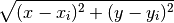
- The distance of a location (x, y) from satellite i is given by the Pythagorean Theorem:
- The “mismatch” between a satellite i and a location (x, y) is the difference between the calculated distance to the satellite and the distance the satellite says it should be:

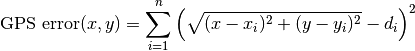
We want to make sure that errors are always positive, so the mismatch is squared when calculating the total error across all the satellites. If there are n satellites in total, this is given by:
Finding the correct location (x, y) is now an optimization problem.
- We want to find the location (x, y) that minimizes this GPS error.
- The stumbledown algorithm with reducing step sizes solves optimization problems.
- Applying the stumbledown algorithm to the “GPS error” function should find the correct location.
The data  for each satellite is available below. These numbers are the ones that should be used in the GPS error function.
| Satellite | X coordinate | Y coordinate | Distance |
| Clueless | 567 | 390.7 | 366.9 |
| Cunningham Muffins | 73.2 | 499.5 | 444.9 |
| Justice League | 204 | 501 | 386 |
| Left 2nd Row Back Table | 337.3 | 609.3 | 480.5 |
| Spaghett | 368.5 | 116.3 | 57.0 |
Report Description
This report consists of the following activities:
Exercise 1. The “Stumble Down” Algorithm
As we covered in class, the “stumble down” algorithm consists of repeatedly taking a random step from a current position and only accepting those steps that are “better” than the current position.
- Describe and implement this algorithm, and use it to find the minimum of the function
 .
.
Note
Write a function
stumbledown(f, p, stepsize, nsteps)where:- f is the function to minimize
- p is the initial point
- stepsize is the maximum step size
- nsteps is the number of steps to try
This function should return a 2D array where the rows correspond to every step that was tried. The rows will contain the values [x, y, f(x, y), success] (success equals 1 if the new position is better than the previous one and 0 otherwise).
Tip
Representing positions using a 2 element NumPy array (for the x and y values) can help to simplify the code.
- Write a
print_stumbledownfunction to print the steps generated by the stumbledown function. For each step this should print the step number, if the step was a success or failure, and the values x, y, and f(x, y).
Exercise 2. The “Stumble Down with Reducing Step Sizes” Algorithm
The “stumble down with reducing step sizes” algorithm keeps track of the number of steps tried, and reduces the step size after a given number of consecutive failures.
- Describe and implement this algorithm, and use it to find the minimum of the function .
Note
Write a function
stumbledown_reducing(f, p, stepsize, nsteps)where:- f is the function to minimize
- p is the initial point
- stepsize is the initial maximum step size
- nsteps is the maximum number of steps to try
This function should return a 2D array where the rows correspond to every step that was tried. The rows will contain the values [x, y, f(x, y), success].
Experiment with and decide for yourself:
- how many failing steps to tolerate,
- what factor to reduce the step size by,
- the tolerance to use as a stopping criterion (just continue while step size > tolerance).
Write a
plot_stumbledownfunction to plot the steps.- Use contourf to plot the level curves of the function
 .
. - On the same graph, plot the steps taken by the algorithm as it approaches the minimum, and the final location.
- Use contourf to plot the level curves of the function
Tip
The algorithm generates a sequence of locations. Each time we accept a new location, we can draw a line from the previous best location to the new best location. This will show the path that the algorithm takes as it approaches the minimum. The successful steps can be sliced out of the results using a Boolean array index.
Exercise 3. The Global Positioning System
- Explain how GPS works. A brief but understandable description of the main concepts is sufficient.
- Apply the “stumble down with reducing step sizes” algorithm to find the optimum location for the 2D version of the GPS problem to 8 significant figures.
Tip
Define a gps_error(x, y) function. This will return the error for a given position (x, y) based on the mismatch between the calculated distance to each satellite and the distances the satellites are reporting.
- Use NumPy 2D arrays to represent the satellite information, one satellite per row.
- Use NumPy array operations to calculate and sum the mismatch error for each satellite without using “for” loops.
- The
stumbledown_reducingfunction accepts a function name as an argument. Finding the optimum location can be accomplished by callingstumbledown_reducingwithgps_erroras this argument.
- Plot the steps taken by the algorithm as it approaches the minimum, and the final location.
Tip
A circle of radius d centered on a point (x, y) can be plotted as follows (‘ec’ is the edge color):
gca().add_patch(Circle((x,y), radius=d, fc='none', ec='c'))
This can be used to plot a circle around each satellite where the radius is the reported distance to the satellite. The correct location should lie at the intersection of these circles.
Exercise 4 (Extra Credit). The Nelder-Mead Algorithm
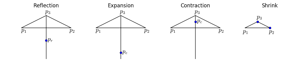
The Nelder-Mead algorithm is another iterative algorithm that makes use of function values at certain points. It keeps track of the vertices of a “simplex” - an n-dimensional tetrahedron - which it attempts to “roll down” the function surface.
For a function f of two variables, the simplex is a triangle with vertices  . The algorithm proceeds by the following steps. Each time a new point is found to replace the “worst” point
  , the algorithm returns to the “Order” step and repeats.
- Order
- Order the vertices of the triangle so that
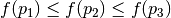 .
.
- Order the vertices
- Reflection
- Take and reflect it through the opposite edge to create a “reflected” point
 .
. - If
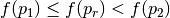 , replace with .
- Take
- Expansion
- If
 , create an “expanded point”
  further out along the line of reflection.
 - If
 , replace with . Otherwise, replace with .
- If
- Contraction
- If
 , create a “contracted point”
  inside the triangle along the line of reflection.
 - If
 , replace with .
- If
- Shrink
- If nothing else has worked, keep
 and shrink the simplex by a given factor towards this vertex.
- If nothing else has worked, keep
You can repeat the algorithm either for a certain number of steps, or until the simplex has shrunk below a certain size.
The steps are summarized in the image below:
For extra credit:
Implement the Nelder-Mead algorithm and apply it to the GPS error function to find the optimum location. Standard values to use are:
- A reflection factor of 1 to find .
- An expansion factor of 2 to find .
- A contraction factor of 1/2 to find .
- A shrink factor of 1/2 to shrink the simplex.
Note
There are different versions of this algorithm. You can look at Wikipedia for further detail on the one described here.
Tip
Implementing the algorithm will be a lot easier if points are represented using two element NumPy arrays (for the x and y values).