Special Relativity Boot Camp
Web edition

This work is licensed under a
Creative Commons Attribution-ShareAlike 4.0 International License
.
Web edition
This work is licensed under a
Creative Commons Attribution-ShareAlike 4.0 International License
.
These lecture notes form a two- to three-week intensive unit on Special Relativity. The notes present relativity as a fundamentally geometric theory, introducing Minkowski space as a metric space from the outset. The Lorentz transformation then follows from invariance of the Minkowski inner product, replacing the traditional algebra based on the \(\beta\) and \(\gamma\) factors with hyperbolic trigonometry and treating the rapidity \(\xi\) as the basic variable. Standard topics such as time dilation, length contraction, the twin paradox, and the ladder-and-barn paradox are then understood geometrically using spacetime diagrams. The notes conclude with a geometric treatment of accelerated reference frames, including the Bell rocket problem and the Rindler horizon.
There is no royal road to geometry.
EuclidYou will learn by the numbers. I will teach you.
Gunnery Sergeant Hartman, Full Metal JacketAfter years of teaching relativity and cosmology at both the undergraduate and graduate levels, I have come to a somewhat dismal conclusion: students in modern physics programs are generally poorly prepared in the Special Theory of Relativity. The reasons for this are not entirely clear, but I suspect two main forces at work. Physicists whose research centers on relativity tend to view Special Relativity as mostly trivial and not worth spending much time on. Physicists whose research lies elsewhere often regard it as peripheral, and likewise not worth spending much time on. As a result, Einstein’s theory is often relegated to a short unit in the required electromagnetism course. It is taught more as an afterthought than as a subject worthy of study in its own right. This does students a disservice. The Special Theory of Relativity is one of the most beautiful and historically significant theories in physics, and it forms an essential foundation for an understanding of quantum fields and gravity. Even in “modern physics’’ electives, we typically present the subject as if it were 1926, not 2026, ignoring a century of accumulated insight and presenting a theory of clocks on trains, metal rods, and riding beams of light. Students are left with a confusing mess of arbitrary rules and algebra that conceals the essential elegance and beauty of the theory, and consequently move on carrying many deep misconceptions. These students then become professors, and the cycle continues of students being poorly taught by professors who themselves were poorly taught, with at best a shallow understanding of the theory. This becomes a problem when students move on to the study of relativistic quantum field theory, General Relativity, and cosmology.
These lecture notes are my own attempt to cope with that problem. I developed these notes as a two- to three-week intensive unit at the beginning of courses in General Relativity and Cosmology, to bring students up to speed on a modern understanding of Special Relativity. Suited to this philosophy, I began calling it a “boot camp,’’ and I have kept the title here. I have by now given these lectures many times, so they have been refined through use in the classroom. The guiding philosophy is a laser focus on relativity as a geometric theory. Almost all problems in relativity can be substantially simplified by replacing the traditional algebraic approach based on the \(\beta\) and \(\gamma\) factors with hyperbolic trigonometry, treating the rapidity \(\xi\) as the basic variable. I present relativity from the outset as a metric theory, with the invariance of the inner product on Minkowski space treated as fundamental, and the Lorentz transformation presented as the hyperbolic analog of orthogonal rotations in Euclidean space. The mathematical setup requires a little more effort up front, but once students have that in hand, concepts like time dilation and length contraction follow completely naturally as geometric properties of trajectories in Minkowski space. I then apply the geometric approach to the twin paradox and the ladder-and-barn paradox, which can be understood intuitively in terms of spacetime diagrams and Lorentz invariance, without thickets of algebra getting in the way. The boot camp concludes with the more advanced topic of accelerated reference frames, demonstrating that the geometric approach to Minkowski space can elegantly handle difficult topics like the Bell rocket problem and the Rindler horizon, all without resorting to a non-Minkowski metric or General Relativity.
These notes are suitable for advanced undergraduate students, beginning graduate students, and even the sophisticated lay reader. It is my hope that they will make at least a small contribution to improving the state of pedagogy on the subject of Special Relativity.
A companion Mathematica notebook containing interactive versions of Figures 14–19 and 21 is available at https://doi.org/10.5281/zenodo.21419218.
In this section, we introduce the concept of the metric, which defines the inner product in a vector space, and use the metric to define a geometric representation of the four-dimensional spacetime of Special Relativity.
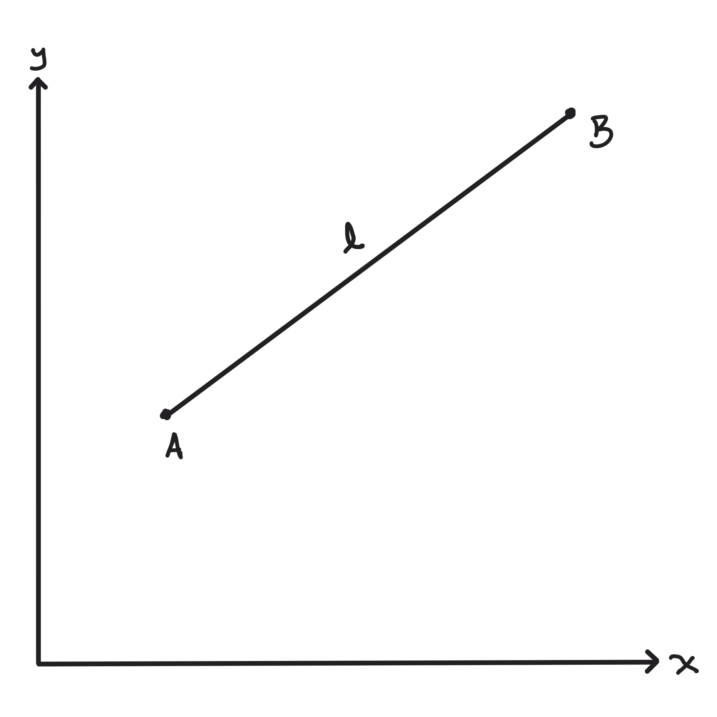
Consider two points \(A\) and \(B\) on a plane, separated by a distance \(\ell\) (Figure 1). This distance is a perfectly well-defined quantity without any sort of coordinate system applied. One can measure the distance from \(A\) to \(B\), for example, with a ruler. The distance between the points is a coordinate invariant.
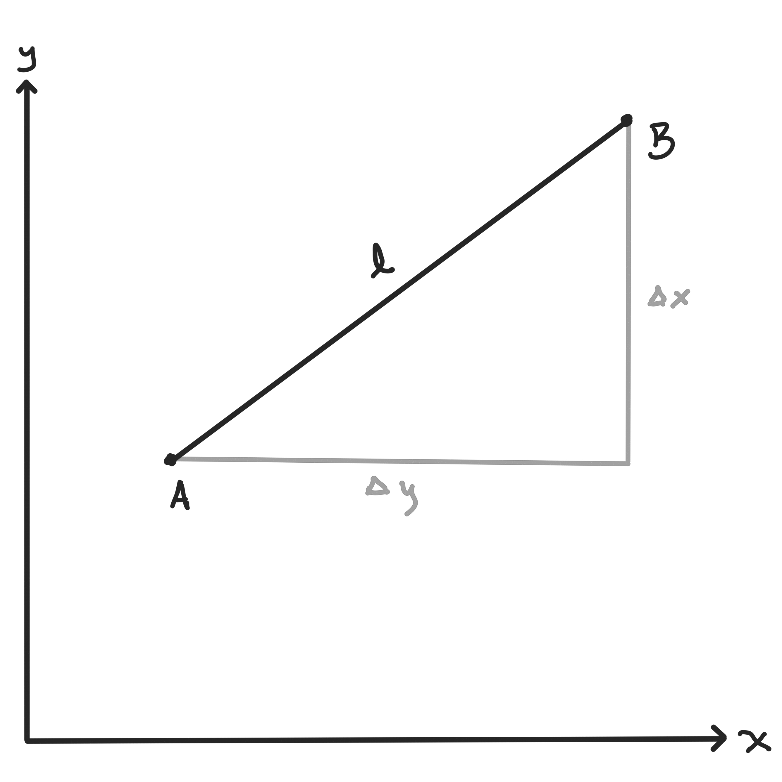
We are, however, free to add a coordinate system on the plane, defined in any way we like (Figure 2). We can then express the length \(\ell\) using Pythagoras’ Theorem,
\[\tag{1} \ell^2 = \Delta x^2 + \Delta y^2. \]
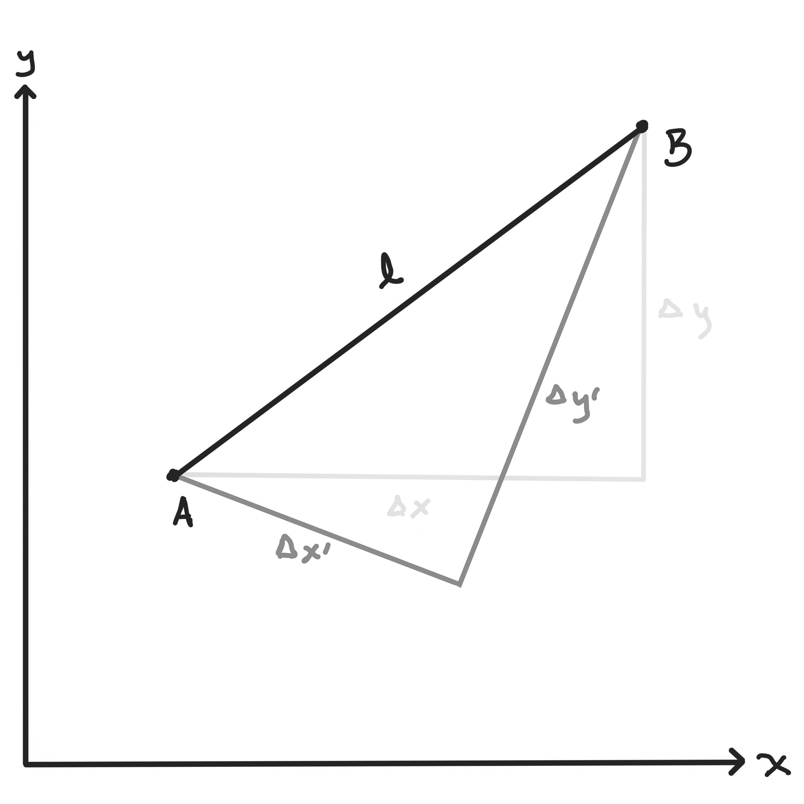
Since \(\ell\) is a coordinate invariant, it doesn’t matter which coordinate system we choose. We could just as easily pick a coordinate system \((x',y')\) which is tilted with respect to our original coordinate system (Figure 3). The length \(\ell\) doesn’t change, so we must therefore have
\[\tag{2} \ell^2 = \Delta x^2 + \Delta y^2 = \left(\Delta x'\right)^2 + \left(\Delta y'\right)^2. \]
The concept of a coordinate-invariant length will be key in our discussion of Special Relativity.
We can write this all in shorthand as a matrix equation,
\[\tag{3} \ell^2 = \sum_{i,j = 1}^2 g_{i j} \left(\Delta x^i\right) \left(\Delta x^j\right), \]
where we have redefined our coordinates as \((x,y) \rightarrow (x^1,x^2)\), where the superscripts are numerical coordinate indices (not exponents!) and the matrix \(g\) is the identity matrix,
\[\tag{4} g_{i j} = \begin{pmatrix} 1 & 0\\ 0 & 1 \end{pmatrix}. \]
It is straightforward to generalize the invariant length defined in Eq. (3) to a definition of a dot product, or an inner product between two vectors \(\mathbf{x} = \left(x^1, x^2\right)\) and \(\mathbf{w} = \left(w^1, w^2\right)\) as:
\[\tag{5} \mathbf{x} \cdot \mathbf{w} \equiv \sum_{i,j = 1}^2 g_{i j} x^i w^j = x^1 w^1 + x^2 w^2. \]
Like the invariant length (3), the inner product between two vectors is a coordinate invariant, and the invariant length is just the inner product of a vector with itself,
\[\tag{6} \ell^2 = \mathbf{x} \cdot \mathbf{x}. \]
Although this notation may seem unnecessarily complicated, it allows us to generalize the concept of distance to much more general spaces than the Euclidean plane. The simplest generalization of this is to a three-dimensional Euclidean space, with vectors \(\mathbf{x}\) and \(\mathbf{w}\), with inner product
\[\tag{7} \mathbf{x} \cdot \mathbf{w} \equiv \sum_{i,j = 1}^3 g_{i j} x^i w^j = x^1 w^1 + x^2 w^2 + x^3 w^3. \]
where our metric is now a 3-by-3 identity matrix,
\[\tag{8} g_{i j} = \begin{pmatrix} 1 & 0 & 0\\ 0 & 1 & 0\\ 0 & 0 & 1 \end{pmatrix}. \]
This is easy to extend to higher-dimensional spaces: for vectors \(\mathbf{x} = \left(x^1, \ldots, x^N\right)\) in an \(N\)-dimensional Euclidean space,
\[\tag{9} \mathbf{x} \cdot \mathbf{w} \equiv \sum_{i,j = 1}^N g_{i j} x^i w^j = x^1 w^1 + \cdots + x^N w^N, \]
with the metric now just an \(N\)-by-\(N\) identity matrix,
\[\tag{10} g_{i j} = \begin{pmatrix} 1 & 0 & 0 & 0 & \ldots\\ 0 & 1 & 0 & 0 & \ldots\\ 0 & 0 & 1 & 0 & \ldots\\ \vdots & \ & \ & \ddots & \ & \ \end{pmatrix}. \]
This can be further generalized to non-Euclidean spaces by specifying a different matrix \(g_{i j}\) as the metric, i.e. a matrix which is not the identity matrix, but some other symmetric matrix. This leads to a general definition of the metric on a vector space:
Definition: Metric
For vectors \(\mathbf{x} = \left(x^1, \ldots,
x^N\right)\), \(\mathbf{w} = \left(w^1,
\ldots, w^N\right)\) in a space of dimension \(N\), the metric is the symmetric
\(N \times N\) matrix \(g_{i j}\) which defines the inner
product
\[\tag{11} \mathbf{x} \cdot \mathbf{w} \equiv \sum_{i,j = 1}^N g_{i j} x^i w^j. \]
In the next section, we introduce the fundamental postulate of Special Relativity, which we reformulate in terms of the inner product in a non-Euclidean space.
We state the fundamental postulate of Special Relativity as follows:
Definition: Inertial Observer
An inertial observer is an observer who is not undergoing an
acceleration.
Definition: Inertial Reference Frame
An inertial reference frame is a choice of coordinate system
for which a particular inertial observer appears to be at rest.
Principle of Relativity
The speed of light is the same in all inertial reference frames.
We define an inertial reference frame to be the rest frame of an unaccelerated observer, i.e. an observer who is weightless. Note that the definition of an inertial observer is an entirely local one: an observer can tell whether or not he is an inertial reference frame without making reference to any other observers. If the observer is weightless, then he is in an inertial reference frame. If the observer is not weightless, he is in a non-inertial reference frame. Absent a gravitational field, an inertial observer travels in a straight line with constant velocity when viewed by any other inertial observer.
To see what the Principle of Relativity means physically, consider a light wave moving a way from a stationary source:
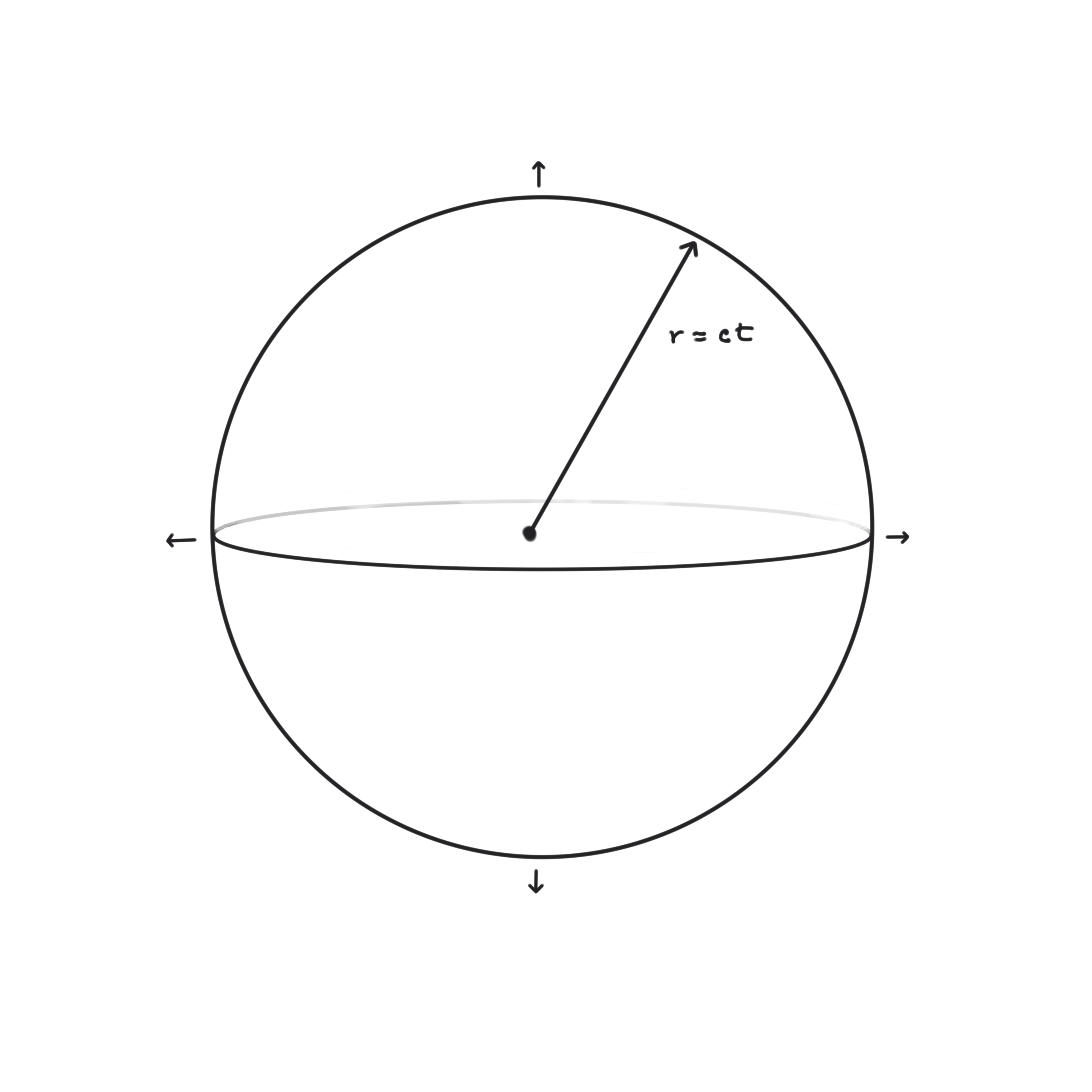
The wave travels outward on a spherical wavefront with radius determined by the speed of light multiplied by the time since emission of the wave:
\[\tag{12} r = c t \]
The Principle of Relativity tells us that this quantity is invariant under transformations between inertial reference frames. This means that
\[\tag{13} c^2 t^2 - r^2 = 0 \]
for all inertial observers: any inertial observer, regardless of motion, sees the light wave moving away from the source in a sphere expanding at the speed of light. (We state this invariant quadratically for reasons that will become clear shortly.)
To interpret this invariance principle geometrically, we extend the three-dimensional Euclidean space of Newtonian physics to a four-dimensional spacetime, with vectors
\[\tag{14} x = \left(x^0, x^1, x^2, x^3\right) = \left(c t, \mathbf{x}\right), \]
where \(\mathbf{x} = \left(x^1, x^2, x^3\right)\) is the position vector in a three-dimensional Euclidean space.
Definition: Four-vector
A four-vector is a vector \(x =
\left(x^0, x^1, x^2, x^3\right) \equiv \left(c t,
\mathbf{x}\right)\) in four-dimensional spacetime.
In what follows we will use the convention that we denote vectors in 3-space with bold (\(\mathbf{x}\)), and in four-space without bold (\(x\)). It is worth noting the units: \(c t\) is a distance, and therefore is in the same units as the spatial coordinates. In what follows, we will adopt the simplifying convention of setting the speed of light to unity, \(c = 1\). This is just a choice of units of measurement: if we measure time in years, we can then measure spatial distances in light-years, so that the speed of light is one light-year per year, or \(c = 1\). If we measure time in seconds, then we likewise measure spatial distances in light seconds, or in units of \(3 \times 10^8\ {\rm m}\). Thus the speed of light \(c\) will disappear from our equations, although it is always implicitly present, and can be recovered by dimensional analysis.
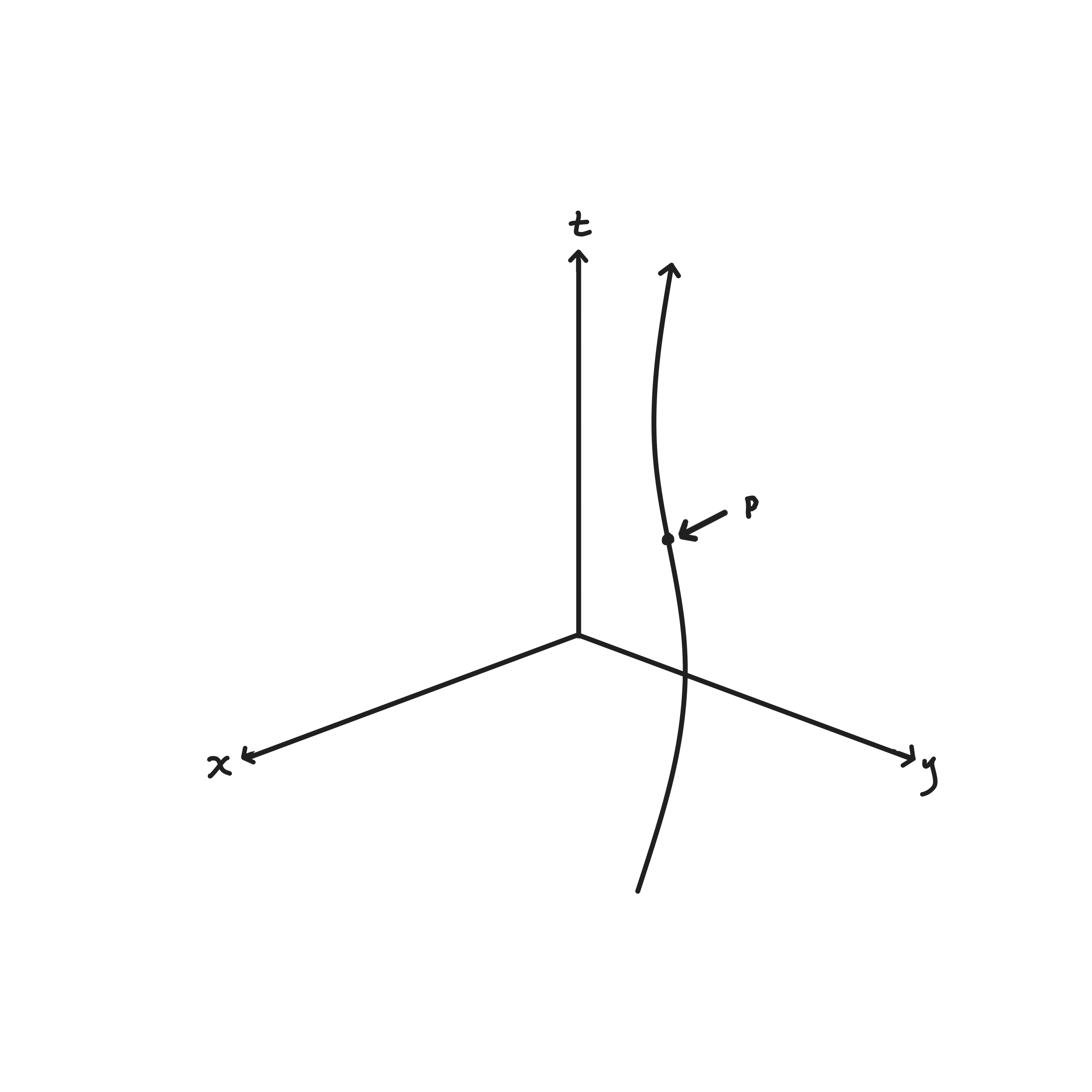
Now consider a particle evolving in time. A particle traveling along a path \(\mathbf{x}\left(t\right)\) traces out a line in spacetime, referred to as a world line (Fig. {5). Any point \(P\) along that path is called an event: an example of an event is the explosion of a supernova, or Neil Armstrong stepping on the Moon, the moment of your birth, or (at the other end of the world line) your death. The concept of a world line can be extended to higher-dimensional objects evolving in time, world sheets and world volumes, as the paths through spacetime of one-dimensional and two-dimensional objects, respectively.
Definition: Event
An event is a point in spacetime.
Definition: World Line
A world line is a one-dimensional connected path in spacetime
corresponding the evolution of a point object in time.
Now consider the path of the light front (13). The moment of emission of the light front is a point in spacetime (an event), after which the light front expands outward in space, following a path \(r(t) = t\): light travels along \(45^\circ\) lines in spacetime, and the spherical light front sweeps out an expanding region, called the light cone (Fig. 6).
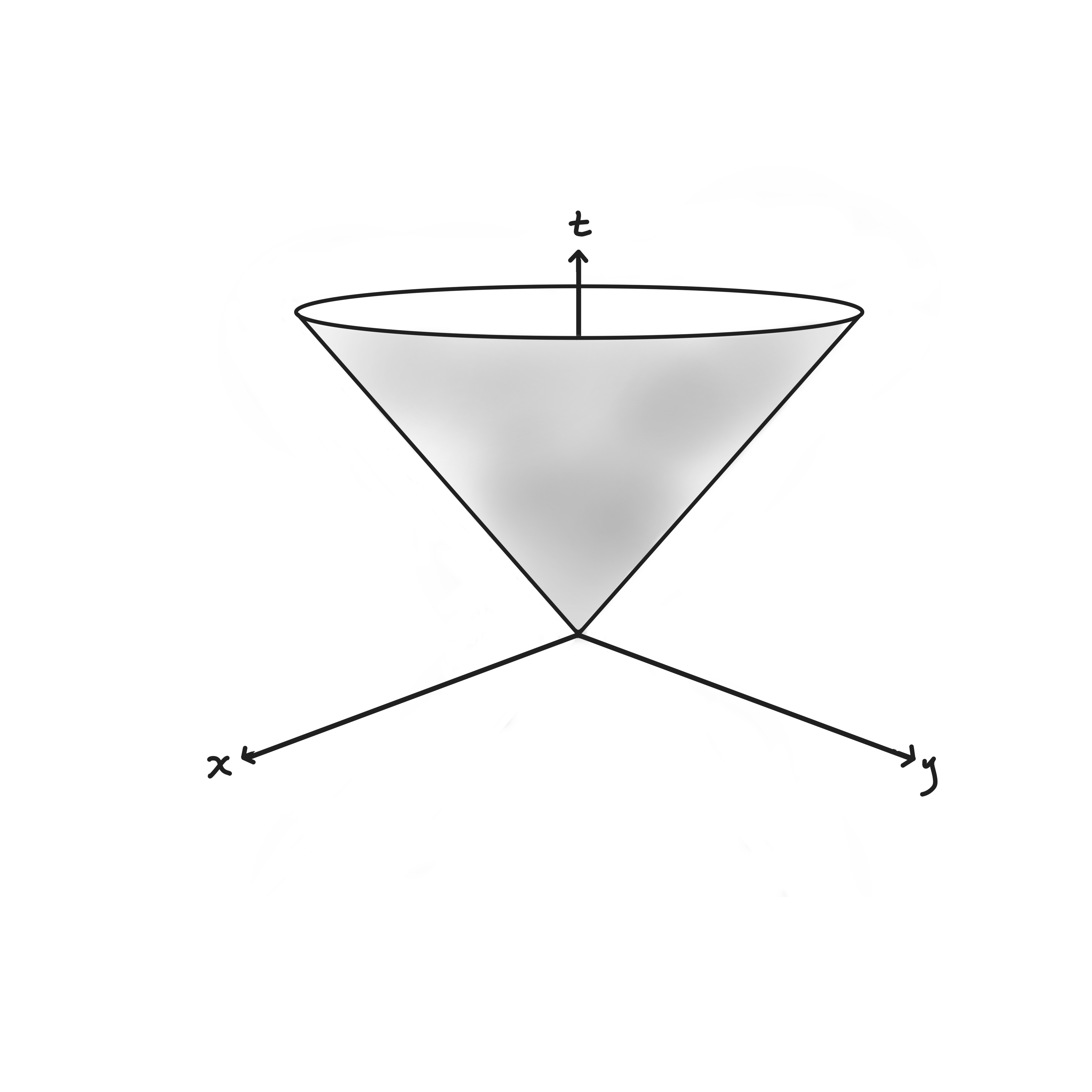
Phrased geometrically, the Principle of Relativity states that photons (or any other massless particles) always move on \(45^\circ\) lines on a plot of spacetime. Furthermore, this is true when viewed from the reference frame of any inertial observer, and it is this invariance which distinguishes relativistic physics from Newtonian physics. This independence of coordinate system suggests an analogy with the invariant length 2.1 in three-dimensional Euclidean space. In the four-dimensional spacetime, we define the squared length of a four-vector \(x = \left(x^0, x^1, x^2, x^3\right) \equiv \left(t, x, y, x\right)\) as:
\[\tag{15} x \cdot x = \sum_{\mu, \nu = 0}^3 \eta_{\mu \nu} x^\mu x^\nu = t^2 - x^2 - y^2 - z^2, \]
where the metric \(\eta_{\mu \nu}\) is given by
\[\tag{16} \eta_{\mu \nu} = \begin{pmatrix} 1 & 0 & 0 & 0\\ 0 & -1 & 0 & 0\\ 0 & 0 & -1 & 0\\ 0 & 0 & 0 & -1 \end{pmatrix}. \]
Notation
Throughout this paper, we use greek letters to denote spacetime indices,
for example \(\mu,\ \nu = 0,\ldots,3\).
We use Latin indices to indicate spatial indices, \(i,\ j = 1,\ldots,3\).
The metric \(\eta_{\mu\nu}\) is not the identity matrix: Spacetime is non-Euclidean, and defined in this way is referred to as Minkowski space; the metric \(\eta_{\mu\nu}\) is called the Minkowski metric. Note that the purely spatial portion of the metric is just the negative of the identity matrix, and is Euclidean:
\[\tag{17} \eta_{i j} = - \begin{pmatrix} 1 & 0 & 0\\ 0 & 1 & 0\\ 0 & 0 & 1 \end{pmatrix}. \]
Spatial distances in Minkowski space are then just the negative of our usual notion of invariant Euclidean length:
\[\tag{18} \mathbf{x} \cdot \mathbf{x} = - \left[x^2 + y^2 + z^2\right]. \]
Minkowski space is also referred to as a \(3+1\) space: three dimensions of space and one of time. Following our procedure for the Euclidean case, we define the inner product in Minkowski space between two four-vectors \(x\) and \(w\) as
\[\tag{19} x \cdot w \equiv \sum_{\mu, \nu = 0}^{3} \eta_{\mu \nu} x^\mu w^\nu = x^0 w^0 - \mathbf{x} \cdot \mathbf{w}, \]
where \(\mathbf{x} \cdot \mathbf{w}\) is the usual Euclidean dot product of spatial three-vectors. We can then restate the Principle of Relativity in geometric language:
Principle of Relativity
The inner product in Minkowski space is invariant under coordinate
transformations between inertial reference frames.
Note that this is a slightly more restrictive condition than our original statement of the Principle of Relativity, since it applies not only to objects traveling at the speed of light, for which
\[\tag{20} x \cdot x = t^2 - \mathbf{x}^2 = 0, \]
but for all four-vectors, including those for which \(x \cdot x \neq 0\). In the next section, we will discuss the physical interpretation of the invariant length in Minkowski space.
While the invariant length \(\ell\) in a Euclidean space has a directly intuitive physical interpretation, the invariant length \(x \cdot x\) in Minkowski space is not so intuitive. What do we mean physically by a “length’’ in a \(3+1\)-dimensional spacetime? Consider a point particle traveling along a world line in spacetime: between two differentially separated points along the world line, the particle travels an invariant length \(d s\), given by:
\[\tag{21} ds^2 = dx \cdot dx = \sum_{\mu,\nu = 0}^3 \eta_{\mu \nu} dx^\mu dx^\nu = dt^2 - d \mathbf{x}^2. \]
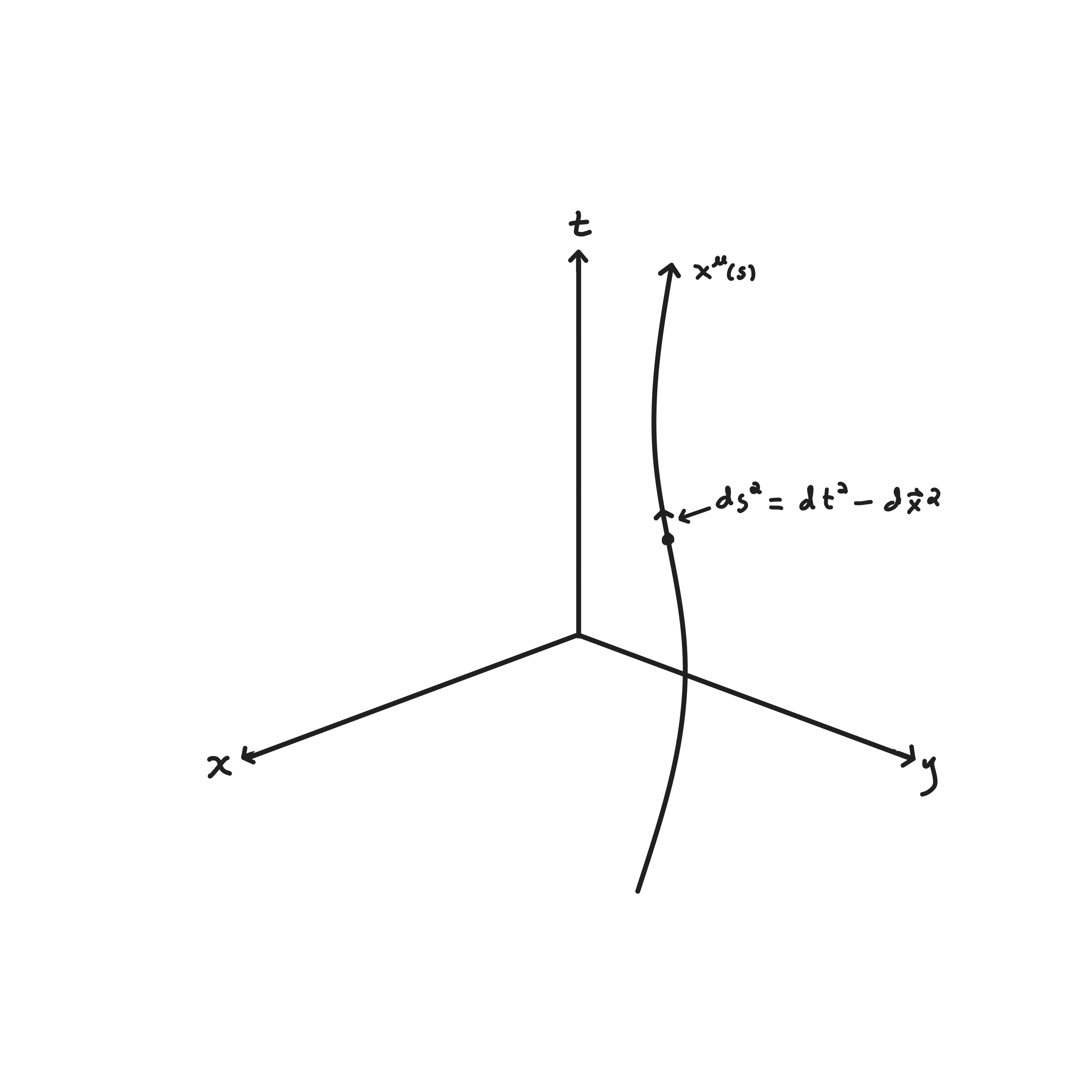
We can then view world lines as connected curves in spacetime parameterized by the invariant length \(s\) measured along the curve, with coordinates \(x^\mu\left(s\right)\) (Fig. 7).
The simplest example of a parameterized world line is the rest frame of an inertial observer: an observer at rest is one whose spatial coordinates are constant, \(d \mathbf{x} = 0\). The world line of the observer at rest is therefore a vertical line in spacetime (Fig. 8), and the invariant length \(s\) is identical to the coordinate time \(t\),
\[\tag{22} ds^2 = dt^2. \]
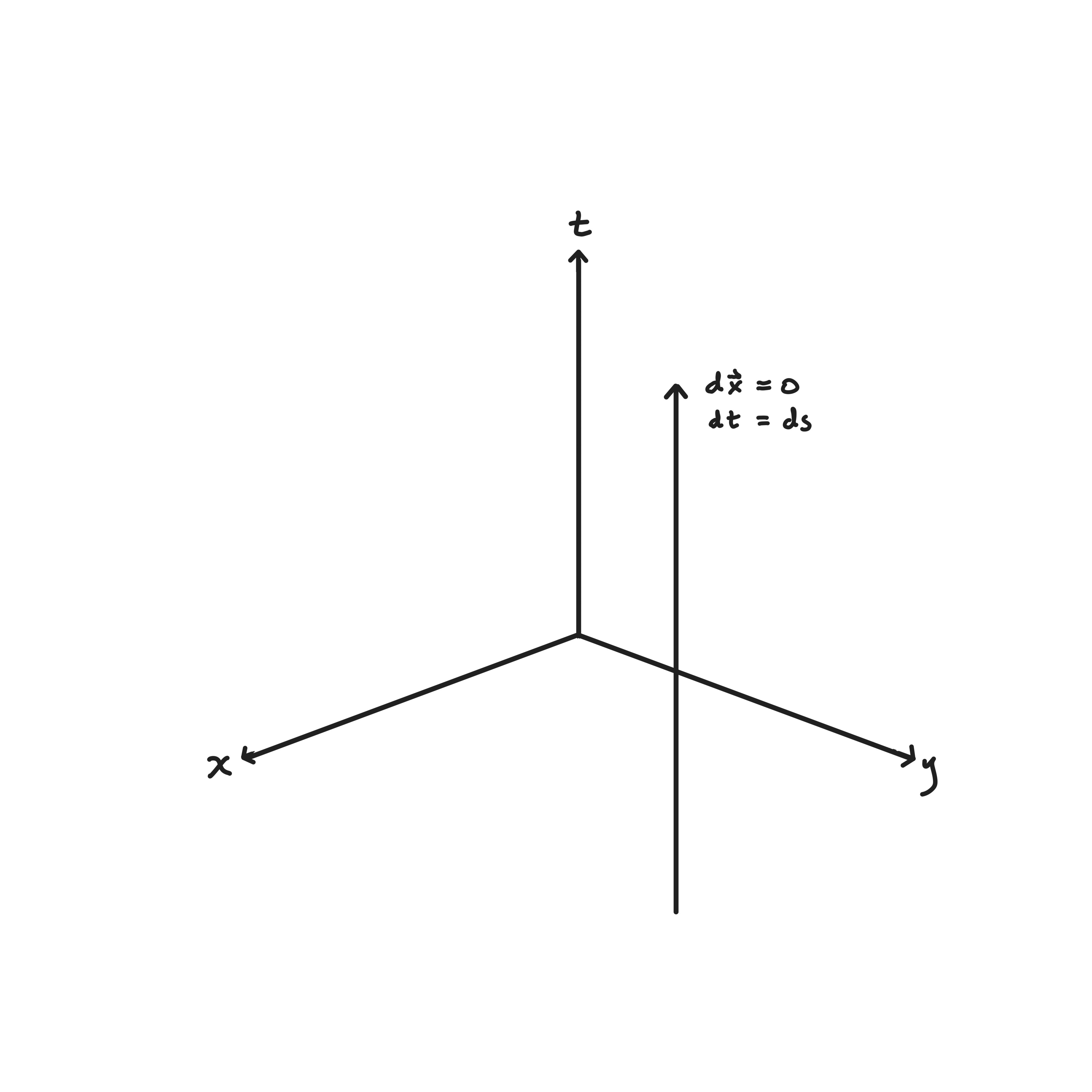
This leads to a simple physical interpretation of the invariant length \(s\) along the world line: it is the time as measured by the observer moving along that world line, called the proper time.
Definition: Proper Time
The proper time \(s\) , given
by the invariant length along a world line, \(ds^2 = dt^2 - d \mathbf{x}^2\), is the time
as measured by an observer traveling along that world line.
Note that in general the world line need not be inertial: for any path through spacetime, including those for accelerated observers, the proper time \(ds\) is identical to the coordinate time \(dt\) in the instantaneous rest frame of the observer, and therefore the integral of the proper time \(d s\) (21) along the world line of an observer
\[\tag{23} \Delta s = \int_{\mathrm{x\left(s\right)}}{d s} \]
is well-defined and is the time measured by that observer along the world line. The proper time \(s\) on a world line is completely independent of reference frame: it is the literal time as measured on a clock carried by a moving observer. This will be important when we discuss accelerated observers in Special Relativity.
The world lines of massless particles like photons are special, since photons propagate on null world lines, for which \(ds = dt^2 - d \mathbf{x}^2 = 0\): particles traveling at the speed of light do not experience time at all, but instead travel along paths of zero proper time. Particles traveling at less than the speed of light, \(\left\vert d \mathbf{x}\right\vert / d t < 1\), by definition travel on paths for which \(dt^2 > d \mathbf{x}^2\), and therefore have proper time \(d s^2 > 0\). But, due to the negative sign in the spatial part of the metric \(\eta_{\mu \nu}\), there is a third possibility: for world lines with \(d \mathbf{x}^2 > d t^2\), which corresponds to particles traveling faster than the speed of light, we have \(d s^2 < 0\) along the world line, which means that the proper time \(d s\) along the world line is an imaginary number. This leads to a categorization of world lines into timelike, spacelike, or null:
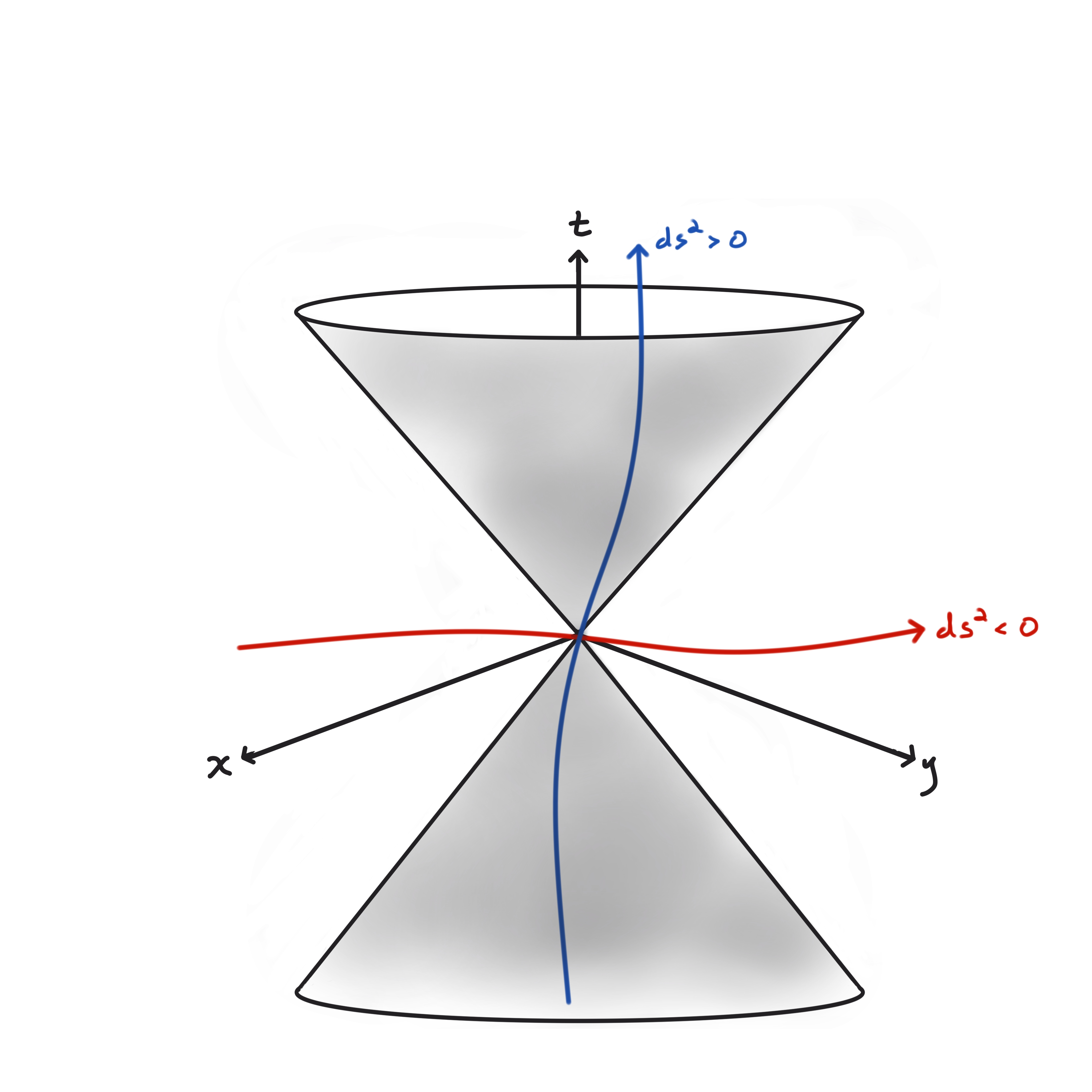
Definition: Timelike World Line
A timelike world line is a path through spacetime with \(ds^2 > 0\).
Definition: Spacelike world line
A spacelike world line is a path through spacetime with \(ds^2 < 0\).
Definition: Null world line
A null world line is a path through spacetime with \(ds^2 = 0\).
All causal paths—that is, all paths for which the proper time is real—are therefore either timelike or null. This leads to a well-defined causal structure for spacetime: Consider an event \(P\): the causal future of \(P\) consists of all timelike or null world lines with \(P\) in their past. Likewise, the causal past of \(P\) consists of all timelike or null world lines with \(P\) in their future. This is shown in Fig. 10. The region which is neither in the future or past of \(P\) is referred to as “Elsewhere’’, and represents the part of spacetime which has no causal connection to \(P\).
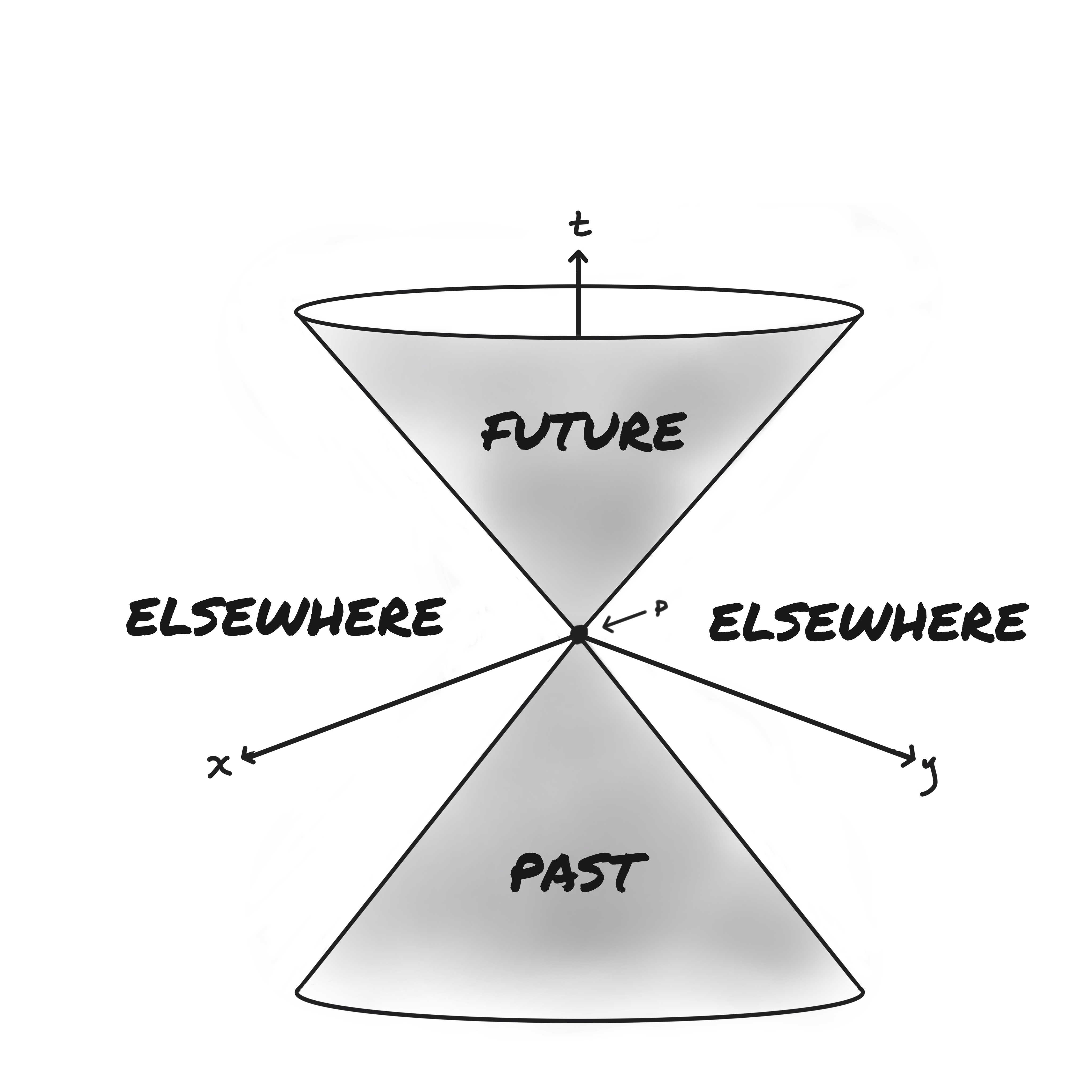
Note that we have added something that was not there before: causal ordering, or defining the direction in spacetime which points toward the future. Unlike the division into timelike and spacelike, causal ordering is not inherent in the metric structure of Minkowski space, which is symmetric under time reversal, \(t \rightarrow -t\). The “arrow of time’’ distinguishing the future from the past is an additional, subtle rule of Special Relativity which is not often remarked upon. The physical origin of the arrow of time is a matter of considerable current debate, with no satisfactory explanation available.
At this point, we have a good picture of the basic geometry of Minkowski space, which is a four-dimensional, non-Euclidean space with properties very different from ordinary Euclidean spaces, including the existence of points separated by imaginary, or spacelike distances. This distance itself has a very different meaning than in a Euclidean space, corresponding to the time as measured along a path between two points (or events) in spacetime. This proper time is defined as a coordinate-invariant inner product on Minkowski space, and it is this invariance that is the key to the physics of Special Relativity. In Section 3, we examine the coordinate invariance of the proper time in detail, leading to the Lorentz transformation between inertial reference frames. In Section 4 we relate this to physical phenomena such as time dilation and Lorentz contraction.
In Section 2, we defined a four-dimensional Minkowski spacetime with vectors
\[\tag{24} x = \left(t, x, y, z\right) = \left(x^0, x^1, x^2, x^3\right) \]
in units where \(c = 1\). The inner product in Minkowski space is defined by
\[\tag{25} x \cdot w \equiv \sum_{\mu,\nu = 0}^3 \eta_{\mu\nu} x^\mu w^\nu, \]
with the metric \(\eta_{\mu\nu}\) defined by:
\[\tag{26} \eta_{\mu \nu} = \begin{pmatrix} 1 & 0 & 0 & 0\\ 0 & -1 & 0 & 0\\ 0 & 0 & -1 & 0\\ 0 & 0 & 0 & -1 \end{pmatrix}. \]
The length of a four-vector,
\[\tag{27} ds^2 \equiv dx \cdot dx = dt^2 - d \mathbf{x}^2, \]
is physically interpreted as the proper time, or time as measured along a world line parametrized by coordinates \(x^\mu\left(s\right)\). The Principle of Relativity states that the inner product in Minkowski space is a coordinate invariant quantity, and in this section we discuss this coordinate invariance and its physical interpretation.
To understand coordinate invariance of the inner product, let us first consider a simple 2-dimensional Euclidean space, with vectors \((x^1, x^2) = (x, y)\) and metric
\[\tag{28} g_{i j} = \delta_{i j} = \begin{pmatrix} 1 & 0 \\ 0 & 1 \end{pmatrix}. \]
Consider a vector \(\mathbf{r}\) as measured in two different coordinate systems, \[\begin{eqnarray} \mathbf{r} = (x, y),\cr \mathbf{r}' = (x', y'). \end{eqnarray}\]. We can write the new coordinates as a matrix transformation of the old coordinates,
\[\tag{29} \mathbf{r}' = \begin{pmatrix} x'\\ y' \end{pmatrix} = \underline{\Lambda} \mathbf{r} \equiv \begin{pmatrix} \Lambda_{11} & \Lambda_{12}\\ \Lambda_{21} & \Lambda_{22} \end{pmatrix} \begin{pmatrix} x\\ y \end{pmatrix}. \]
We can represent this matrix transformation in index form by
\[\tag{30} \left(r'\right)^i = \sum_{j = 1, 2} \Lambda_{i j} r^j. \]
In general, the transformation matrix \(\underline{\Lambda}\) is completely arbitrary. For example, we could define a transformation which “stretches’’ the x-axis,
\[\tag{31} \underline{\Lambda} = \begin{pmatrix} 2 & 0\\ 0 & 1 \end{pmatrix} \]
so that under the transformation,
\[\tag{32} \left(x, y\right) \longrightarrow \left(2 x, y\right), \]
which is a well-defined invertible mapping of \(\mathbb{R}^2 \rightarrow \mathbb{R}^2\). However, we wish to consider a special set of coordinate transformations which leave the lengths of vectors invariant:
\[\tag{33} \mathbf{r}' = \underline{\Lambda} \mathbf{r}\ :\ \left\vert\mathbf{r}'\right\vert = \left\vert\mathbf{r}\right\vert\ \forall \mathbf{r}. \]
More generally, we can define an orthogonal transformation as follows:
Definition: Orthogonal Transformation
An orthogonal transformation on a Euclidean vector space \(\mathbb{R}^D\) is a linear transformation
which leaves the inner product invariant: \[\begin{eqnarray}
\mathbf{r}' \cdot \mathbf{s}' &=& \sum_{i,j =
1}^{D}{\delta_{i j} \left(r'\right)^i \left(s'\right)^j}\cr
&=& \sum_{i,j = 1}^{D}{\delta_{i j} r^i s^j}\cr
&=& \mathbf{r} \cdot \mathbf{s}\ \forall \mathbf{r}, \mathbf{s}
\in \mathbb{R}^D,
\end{eqnarray}\] where
\[\tag{34} \mathbf{r}' = \underline{\Lambda} \mathbf{r},\ \mathbf{s}' = \underline{\Lambda} \mathbf{s}. \]
We can write an orthogonal transformation in index form,
\[\tag{35} \left(r'\right)^i = \sum_{j = 1}^{D}{\Lambda_{i j} r^j}, \]
so that the transformation of the inner product is then \[\begin{eqnarray} \mathbf{r}' \cdot \mathbf{s}' &=& \sum_{i, j}{\delta_{i j} \left(r'\right)^i \left(s'\right)^j} \cr &=& \sum_{i, j}{\delta_{i j} \left[\sum_{k}{\Lambda_{i k} r^k}\right] \left[\sum_{\ell}{\Lambda_{j \ell} s^\ell}\right]}. \end{eqnarray}\] Rearranging sums results in the expression
\[\tag{36} \mathbf{r}' \cdot \mathbf{s}' = \sum_{k, l}{\left[\sum_{i, j} \delta_{i j} \Lambda_{i k} \Lambda_{j \ell}\right] r^k s^\ell}. \]
However, orthogonality requires \[\begin{eqnarray} \mathbf{r}' \cdot \mathbf{s}' = \mathbf{r} \cdot \mathbf{s} &=& \sum_{k, \ell}{\delta_{k \ell} r^k s^\ell} \cr &=& \sum_{k, l}{\left[\sum_{i, j} \delta_{i j} \Lambda_{i k} \Lambda_{j \ell}\right] r^k s^\ell}, \end{eqnarray}\] which requires
\[\tag{37} \delta_{k \ell} = \sum_{i, j}{\delta_{i j} \Lambda_{i k} \Lambda_{j \ell}}. \]
That is, orthogonality of the transformation \(\underline{\Lambda}\) requires that the metric \(\delta_{i j}\) be invariant under the transformation (37). The invariance of the inner product is equivalent to the invariance of the metric!
Using the 2-D Euclidean metric (28) as an example, the condition (37) results in a system of simultaneous equations for the four elements of the transformation matrix \(\underline{\Lambda}\), \[\begin{eqnarray} &&\Lambda_{11}^2 + \Lambda_{21}^2 = 1,\cr &&\Lambda_{11} \Lambda_{12} + \Lambda_{21} \Lambda_{22} = 0,\cr &&\Lambda_{12}^2 + \Lambda_{22}^2 = 1, \end{eqnarray}\] with general solution \[\begin{eqnarray} &&\Lambda_{1 1} = \Lambda_{2 2} = \cos{\theta},\cr &&\Lambda_{1 2} = -\Lambda_{2 1} = -\sin{\theta}. \end{eqnarray}\] The transformation \(\underline{\Lambda}\) is then just the familiar rotation matrix,
\[\tag{38} \underline{\Lambda} = \begin{pmatrix} \cos{\theta} & -\sin{\theta} \\ \sin{\theta} & \cos{\theta} \end{pmatrix}. \]
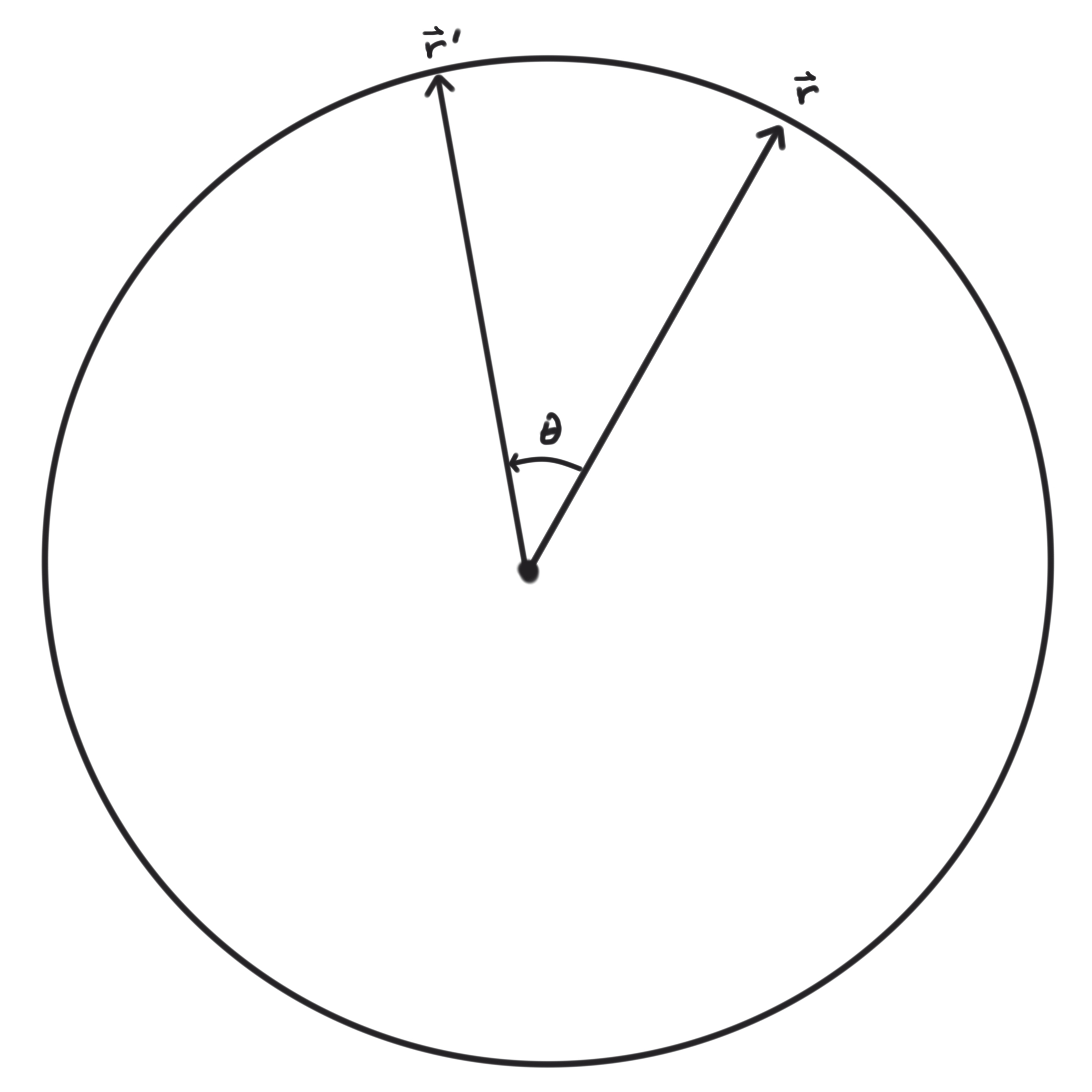
Geometrically speaking, an orthogonal transformation \(\underline{\Lambda}\) maps a vector \(\mathbf{r}\) to another vector \(\mathbf{r}'\) lying on a circle of radius \(\left\vert\mathbf{r}\right\vert\) (Fig. 11): this is the most general transformation which leaves the Euclidean metric invariant.
The generalization to higher-dimensional Euclidean spaces \(\mathbb{R}^D\) is straightforward: An orthogonal transformation maps a vector \(\mathbf{r}\) to another vector \(\mathbf{r}'\) lying on a sphere of dimension \(D - 1\) with radius \(\left\vert\mathbf{r}\right\vert\). (An example in three dimensions is the Euler rotation matrices.) Such transformations form the orthogonal group \(O(D)\).
Consider a set of basis vectors \(\mathbf{e}_i\) on the space, such that they are both of unit length, and mutually orthogonal:
\[\tag{39} \mathbf{e}_i \cdot \mathbf{e}_j = \delta_{i j}. \]
We can then write a vector \(\mathbf{v}\) as a sum of components \(v^i\) multiplying the basis vectors,
\[\tag{40} \mathbf{v} = \sum_i v^i \mathbf{e}_i. \]
The vector \(\mathbf{v}\) is the coordinate-invariant geometric object connecting two points on the plane (Fig. 1). The choice of basis vectors \(\mathbf{e}_i\) defines a coordinate system on the plane, and the numbers \(v^i\) are the coordinates of \(\mathbf{v}\) relative to that choice of basis. We can define a new coordinate system relative to different basis vectors \(\mathbf{e}'{}_i\) by a rotation
\[\tag{41} \mathbf{e}'{}_i = \sum_{j} \Lambda_{j i} \mathbf{e}_j, \]
where \(\Lambda_{j i}\) is an orthogonal matrix (38). Note that this is the transpose of the vector transformation rule (35); by orthogonality, this is the inverse transformation. We next show that this results in the vector components obeying Eq. (35). The vector \(\mathbf{v}\) is coordinate-invariant, but its components are not: relative to the rotated basis \(\mathbf{e}'{}_i\), the coordinates are
\[\tag{42} \begin{aligned} \mathbf{v} = \sum_i \left(v'\right)^i \mathbf{e}'{}_i &= \sum_i \left(v'\right)^i \left(\sum_{j} \Lambda_{j i} \mathbf{e}_j\right) &= \sum_{i,j} \left(v'\right)^i \Lambda_{j i} \mathbf{e}_j &= \sum_j v^j \mathbf{e}_j, \end{aligned} \]
where the last line follows from the invariance of \(\mathbf{v}\) and Eq. (40). The basis vectors \(\mathbf{e}_i\) therefore transform with the orthogonal matrix \(\Lambda_{j i}\) (41). Since the basis vectors \(**e**_i\) are linearly independent, the invariance of \(\mathbf{v}\) requires that the components \(v^i\) transform with the inverse matrix,
\[\tag{43} v^j = \sum_i \Lambda_{j i} \left(v'\right)^i = \sum_i \Lambda^{-1}_{i j} \left(v'\right)^i, \]
where we have used orthogonality, \(\Lambda^{-1}_{i j} = \Lambda_{j i}\). Then
\[\tag{44} \left(v'\right)^i = \sum_j \Lambda_{i j} v^j, \]
which is the vector transformation (35). That is, if we rotate the basis vectors \(\mathbf{e}_i\) clockwise, that is equivalent to a counter-clockwise rotation of the components \(v^i\), and vice-versa. We therefore distinguish these two transformation laws by notation. Components transforming with the basis carry lower indices and are said to transform covariantly; components transforming with the inverse transformation carry upper indices and are said to transform contravariantly. We write covariant components with a “downstairs’’, or subscript index \(\mathbf{e}_i\), and contravariant components with an “upstairs’’, or superscript index \(v^i\). The need for two kinds of indices therefore has nothing to do with the vectors themselves. It arises because basis vectors and coordinate components necessarily transform in opposite ways if the geometric vector is to remain unchanged.
We introduce a simplifying shorthand notation, in which we implicitly represent sums by repeated indices,
\[\tag{45} x \cdot y = \sum_{i j} g_{i j} x^i y^j \equiv g_{i j} x^i y^j. \]
That is, whenever a subscript index is repeated with a superscript index, the index is implicitly summed over. We can convert a contravariant index to a covariant index by summing over the metric,
\[\tag{46} x_i = g_{i j} x^j, \]
so that we can then write the invariant inner product as a sum over covariant and contravariant indices,
\[\tag{47} x \cdot y = g_{i j} x^i y^j = x_j y^j = x^i y_i. \]
This extends to higher-rank tensors as well. A rank-2 tensor \(T\) can be covariant, denoted with two downstairs indices \(T_{i j}\), or contravariant \(T^{i j}\), or mixed, \(T^i{}_j\). In the case of the metric \(g_{i j}\), we define its inverse as a rank-2 contravariant tensor \(g^{i j}\), such that
\[\tag{48} g^{i k} g_{k j} \equiv \delta^i{}_j, \]
where \(\delta^i{}_j\) is the usual identity matrix. We then raise covariant (downstairs) index to a contravariant (upstairs) index using the inverse metric,
\[\tag{49} x^i = g^{i j} x_j. \]
In the case of the Euclidean metric, this is trivial, since the metric itself is the identity matrix, \(g_{i j} = \delta_{i j}\), so that likewise write the inverse metric as an identity \(g^{i j} = \delta^{i j}\), and
\[\tag{50} \delta^{i k} \delta_{k j} = \delta^i{}_j. \]
In the case of a non-Euclidean space, the metric and its inverse need not be the same. The orthogonal transformation matrix \(\Lambda\) is itself a rank-2 tensor, and we can write the vector transformation rule as a sum over a mixed tensor
\[\tag{51} \left(v'\right)^i = \Lambda^i{}_j v^j, \]
where \(\Lambda^i{}_j\) is just the orthogonal matrix (38). Similarly, basis vectors carry covariant indices, and transform as
\[\tag{52} \mathbf{e}'_i = \Lambda^j{}_i \mathbf{e}_j. \]
Rank-2 tensors such as the metric transform as
\[\tag{53} g_{k \ell} = \Lambda^i{}_k \Lambda^j{}_\ell g_{i j}. \]
Orthogonality (37) then requires
\[\tag{54} \Lambda^i{}_k \Lambda^j{}_\ell \delta_{i j} = \delta_{k \ell}. \]
We next consider the case of (non-Euclidean) Minkowski space.
Now let us consider a 2-dimensional spacetime, with one spatial direction and one direction of time. We define vectors in this space \((x^0, x^1) = (t, x)\) and metric
\[\tag{55} g_{\mu \nu} = \begin{pmatrix} 1 & 0 \\ 0 & -1 \end{pmatrix}. \]
This is called a “1+1’’ space. The inner product of two vectors in this space is
\[\tag{56} x \cdot y = \sum_{\mu\nu = 0,1}{x^\mu y^\nu} = x^0 y^0 - x^1 y^1, \]
which defines a non-Euclidean hyperbolic geometry.
We again apply the summation convention, in which repeated indices are implicitly summed over,
\[\tag{57} x \cdot y \equiv \eta_{\mu\nu} x^\mu y^\nu \equiv \sum_{\mu,\nu} \eta_{\mu\nu} x^\mu y^\nu. \]
We will later apply this convention to a full 3+1 spacetime, where repeated indices are summed over \(\mu, \nu = 0, \ldots, 3\), but in our simple 1+1 example, the sums are implicitly over \(\mu, \nu = 0, 1\).
For a given four-vector \(x\) with components \(x^\mu\), we can define a general linear coordinate transformation \(x \rightarrow x'\) as a matrix multiplication
\[\tag{58} \left(x'\right)^\mu = {\Lambda^\mu_{}}_\nu x^\nu, \]
where, by the summation convention, we are implicitly summing over the index \(\nu\). The coordinate transformation matrix \(\Lambda\) is in general an arbitrary, invertible matrix, but we wish to define an analog of the Euclidean orthogonal transformation which preserves the inner product on our hyperbolic spacetime, as follows: \[\begin{eqnarray} \left(x'\right) \cdot \left(y'\right) &=& \eta_{\mu \nu} \left(x'\right)^\mu \left(y'\right)^\nu \cr &=& \eta_{\mu\nu} \left[\Lambda^{\mu}{}_{\lambda} x^\lambda\right] \left[\Lambda^{\nu}{}_{\sigma} y^\sigma\right] \cr &=& \left[\eta_{\mu\nu} \Lambda^{\mu}{}_{\lambda} \Lambda^{\nu}{}_{\sigma}\right] x^\lambda y^\sigma \cr &=& \eta_{\lambda \sigma} x^\lambda y^{\sigma}. \end{eqnarray}\] The middle two lines of the above expression represent quadruple sums, over indices \(\mu\), \(\nu\), \(\lambda\), \(\sigma\), exactly as in Eqs. (??,36). As in the Euclidean case, invariance of the inner product is equivalent to invariance of the metric under the transformation \(\Lambda\),
\[\tag{59} \eta_{\mu\nu} \Lambda^{\mu}{}_{\lambda} \Lambda^{\nu}{}_{\sigma} = \eta_{\lambda \sigma}. \]
For our 1+1 spacetime metric (55), this results in a set of equations for the elements of the matrix \(\Lambda^\mu{}_\nu\), \[\begin{eqnarray} &&\left(\Lambda^{0}{}_{0}\right)^2 - \left(\Lambda^{1}{}_{0}\right)^2 = 1,\cr &&\Lambda^{0}{}_{0} \Lambda^{0}{}_{1} - \Lambda^{1}{}_{0} \Lambda^{1}{}_{1} = 0,\cr &&\left(\Lambda^{0}{}_{1}\right)^2 - \left(\Lambda^{1}{}_{1}\right)^2 = 1, \end{eqnarray}\] with general solution \[\begin{eqnarray} &&\Lambda^{0}{}_{0} = \Lambda^{1}{}_{1} = \cosh{\xi},\cr &&\Lambda^{0}{}_{1} = \Lambda^{1}{}_{0} = \sinh{\xi}. \end{eqnarray}\] We can then write the transformation matrix \(\Lambda^\mu{}_\nu\) in matrix form, in analogy with the orthogonal matrix (38),
\[\tag{60} \Lambda^\mu{}_\nu = \begin{pmatrix} \cosh{\xi} & \sinh{\xi} \\ \sinh{\xi} & \cosh{\xi} \end{pmatrix}. \]
This is the Lorentz transformation, which is the hyperbolic analog of the orthogonal transformation. It is in fact superficially similar, with the trigonometric functions \(\cos()\) and \(\sin()\) replaced by the hyperbolic trig functions \(\cosh()\) and \(\sinh()\), and the rotation angle \(\theta\) replaced by the real number \(\xi\), called the rapidity.
To visualize the Lorentz transformation geometrically, consider a spacelike unit vector
\[\tag{61} x = (t, x) = (0, 1). \]
The invariant length of the vector \(x\) is then
\[\tag{62} x \cdot x = \eta_{\mu \nu} x^\mu x^\nu = -1. \]
Under a Lorentz transformation with rapidity \(\xi\), the vector \(x\) becomes
\[\tag{63} \left(x'\right)^\mu = \Lambda^\mu{}_\nu x^\nu, \]
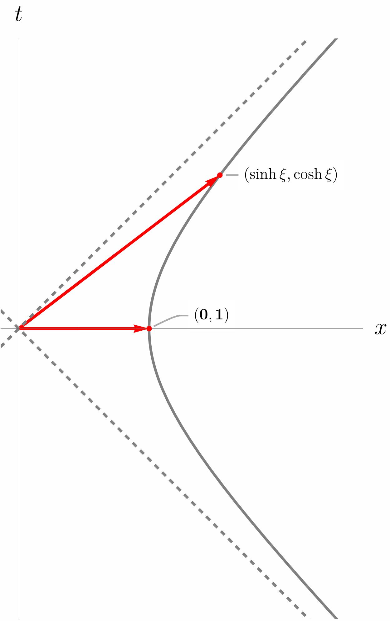
so that \[\begin{eqnarray} &&t' = t \cosh{\xi} + x \sinh{\xi} = \sinh{\xi},\cr &&x' = t \sinh{\xi} + x \cosh{\xi} = \cosh{\xi}. \end{eqnarray}\] So our transformed vector is \(x' = (\sinh{\xi},\cosh{\xi})\), with length
\[\tag{64} x' \cdot x' = \sinh^2{\xi} - \cosh^2{\xi} = -1, \]
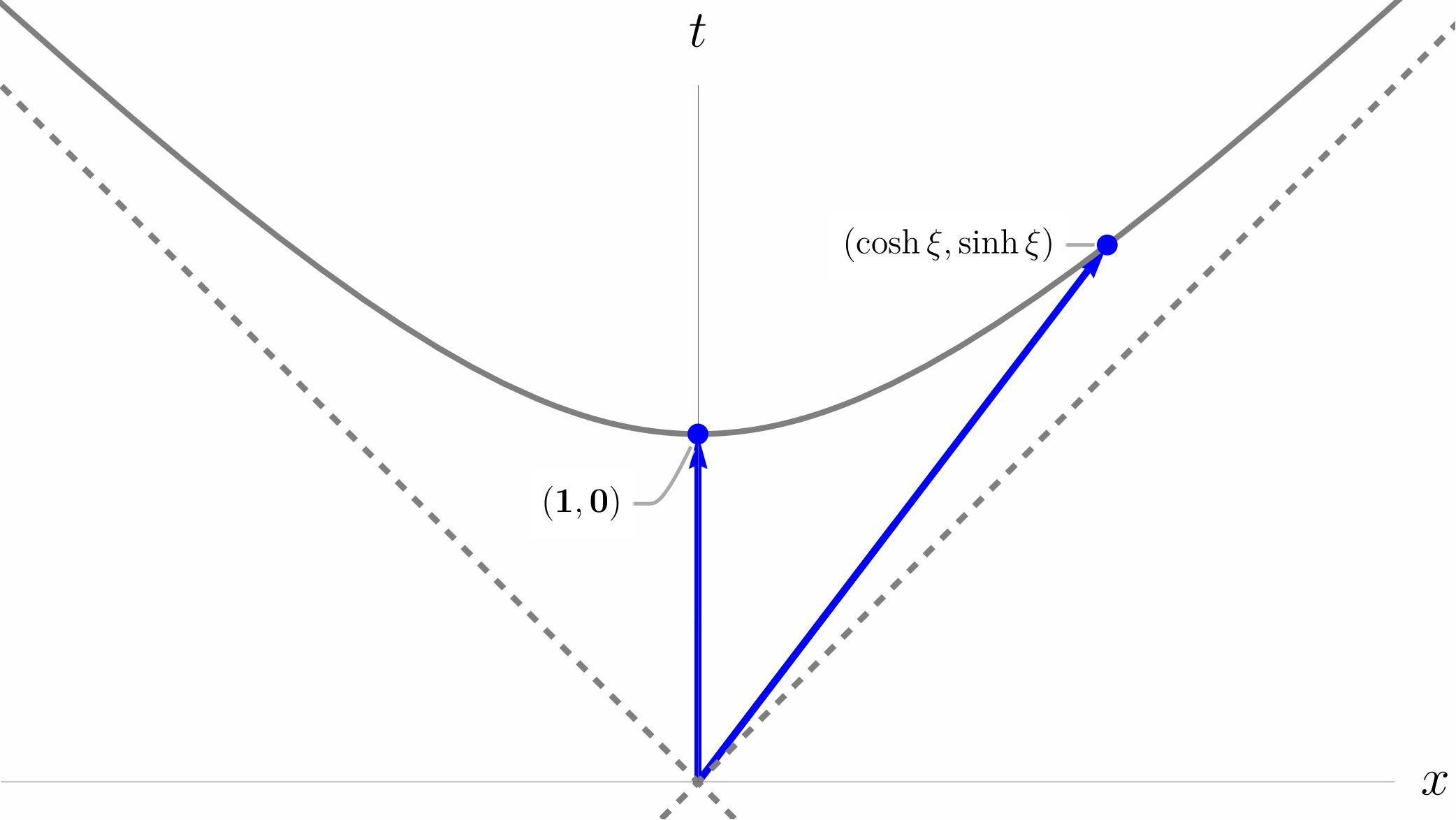
which, as expected, is invariant under the Lorentz transformation: a vector of proper length \(ds^2 = -1\) is mapped by the Lorentz transformation onto another vector with identical proper length (Fig. 12). Similarly, a timelike unit vector with proper length \(ds^2 = +1\) is mapped by the Lorentz transformation onto another timelike unit vector (Fig. 13),
\[\tag{65} x = (1, 0) \rightarrow = x' = \left(\cosh{\xi},\sinh{\xi}\right). \]
This is a direct analog to the orthogonal transformation, which maps a unit vector on the unit circle to to another vector on the unit circle, \(x^2 + y^2 = +1\), (Fig. 11), while in spacetime, vectors are mapped by the Lorentz transformation along unit hyperbolae, \(t^2 - x^2 = \pm 1\). In the full \(3+1\)-dimensional space, the complete symmetry group of invariant transformations is then the Lorentz transformation combined with orthogonal transformations acting on the Euclidean spatial components. When combined with symmetry under spatial translations, these form the Poincaré Group. When looking at diagrams of the Lorentz transformation, it is important to keep in mind that—despite appearances—the transformed vector and the original vector are the same length, as define by the inner product. Spacetime diagrams like Figs. 12 and 13 distort Minkowski space by mapping the hyperbolic manifold to a Euclidean plane.
We have so far treated the Lorentz transformation as a purely geometric object: the symmetry that leaves the inner product on Minkowski space invariant. The Principle of Relativity provides the bridge from geometry to physics: Lorentz transformations map between different inertial reference frames, i.e. the rest-frame coordinate systems of observers moving relative to each other. We connect this geometric picture to the physics of moving observers in the next chapter.
In Section 3, we discussed in detail the geometry of Minkowski space and of the Lorentz transformation, which preserves the spacetime interval,
\[\tag{66} ds^2 = \eta_{\mu \nu} dx^\mu dx^\nu = dt^2 - d \mathbf{x}^2. \]
This is purely geometric; in this section, we connect the geometry to physics. The Principle of Relativity tells us how: because inertial observers see the same speed of light regardless of their velocity, this means that the Lorentz transformation maps between different inertial rest frames. The connection between a choice of rest frame and the corresponding Lorentz transformation is made quantitative by finding a relation between the rapidity \(\xi\) and the velocity \(\mathbf{v}\) of the reference frame. Once we have this relation, we can easily derive the Lorentz transformation that maps between an inertial rest frame and a reference frame moving with relative velocity \(\mathbf{v}\). We begin by defining important concepts such as the four-velocity and four-acceleration, and proving a few useful theorems.
An observer moving through spacetime traces out a world line from the past to the future. We can represent the world line parametrically as a four-vector-valued function \(x^\mu\left(s\right)\) encoding the position of the observer in 3+1-dimensional Minkowski space as a function of the proper time as measured by the observer. A physical observer moves on a world line which is everywhere timelike:
Definition: Physical Observer
A physical observer is an observer whose world line is always
timelike:
\[\tag{67} dx^\mu dx_\mu = ds^2 > 0. \]
Note that a physical observer need not be inertial. We then define the four-velocity as a vector tangent to the world line:
Definition: Four-Velocity
Given a parametric world line \(x^\mu\left(s\right)\), the
four-velocity is defined as the derivative with respect to the
proper time,
\[\tag{68} u^\mu \equiv \frac{d x^\mu\left(s\right)}{d s}, \]
and is tangent to the world line.
Theorem
For any physical observer with four-velocity \(u^\mu\), the four-velocity has unit
norm:
\[\tag{69} u^\mu u_\mu = 1. \]
Proof.
\[\tag{70} \begin{aligned} u^\mu u_\mu &= \eta_{\mu \nu} \frac{d x^\mu}{d s} \frac{d x^\nu}{d s} \\ &= \frac{\eta_{\mu \nu} d x^\mu d x^\nu}{d s^2} \\ &= \frac{d s^2}{d s^2} = 1. \end{aligned} \]
□
Just as we defined the four-velocity as the parametric derivative of the world line \(x^\mu\left(s\right)\), we can define the four-acceleration as the parametric derivative of the four-velocity:
Definition: Four-Acceleration
Given a parametric world line \(x^\mu\left(s\right)\) with four-velocity
\(u^\mu\), the
four-acceleration is defined as the derivative with respect to
the proper time,
\[\tag{71} a^\mu \equiv \frac{d u^\mu\left(s\right)}{d s}. \]
Theorem
For any physical observer with four-velocity \(u^\mu\) and four-acceleration \(a^\mu\), the four-velocity and
four-acceleration are orthogonal:
\[\tag{72} a^\mu u_\mu = 0. \]
Proof. Begin with the normalization of the four-velocity,
\[\tag{73} u^\mu u_\mu = 1. \]
Then,
\[\tag{74} \begin{aligned} \frac{d}{d s}\left(u^\mu u_\mu\right) &= \frac{d u^\mu}{d s}u_\mu + u^\mu \frac{d u_\mu}{d s} \\ &= a^\mu u_\mu + u^\mu a_\mu \\ &= 2a^\mu u_\mu \\ &= 0. \end{aligned} \]
Therefore \(a^\mu u_\mu = a_\mu u^\mu = 0\).
□
We define an inertial observer as one with vanishing four-acceleration:
Definition: Inertial Observer
An inertial observer is a physical observer for whom the
four-acceleration everywhere vanishes:
\[\tag{75} a^\mu\left(s\right) = \frac{d u^\mu}{d s} = \frac{d^2 x^\mu}{d s^2} = 0 \quad \forall s. \]
Lemma
An inertial observer has constant three-velocity,
\[\tag{76} \mathbf{v} = \frac{d \mathbf{x}}{d t} = \text{const.} \]
Proof. We can write the four-acceleration in component form,
\[\tag{77} \begin{aligned} a^\mu = \frac{d u^\mu}{d s} &= \frac{d}{d s}\left[\frac{d t}{d s}\left(1,\mathbf{v}\right)\right] \\ &= \frac{d^2t}{d s^2}\left(1,\mathbf{v}\right) + \frac{d t}{d s}\left(0,\frac{d\mathbf{v}}{d s}\right) \\ &= \frac{d^2t}{d s^2}\left(1,\mathbf{v}\right) + \left(\frac{d t}{d s}\right)^2\left(0,\frac{d\mathbf{v}}{d t}\right) \\ &= 0. \end{aligned} \]
The time component gives
\[\tag{78} \frac{d^2t}{d s^2}=0. \]
The spatial components then reduce to
\[\tag{79} \left(\frac{d t}{d s}\right)^2\frac{d\mathbf{v}}{d t}=0. \]
Since \(d t/d s>0\) for a future-directed physical observer, \(d\mathbf{v}/d t=0\).
□
Definition: Rest Frame
For any inertial observer, the rest frame is the coordinate
system for which the four-velocity is
\[\tag{80} u^\mu = \left(1, 0, 0, 0\right). \]
In the rest frame, the proper time and the coordinate time are identical,
\[\tag{81} \frac{d t}{d s} = 1. \]
We next prove the key theorem that lets us connect geometry to physics: any two inertial reference frames are related by a single Lorentz transformation.
Theorem
Any inertial observer can be transformed into the rest frame by a single
Lorentz transformation.
Proof. Consider an inertial observer moving on a world line with
\[\tag{82} \mathbf{v}\equiv\frac{d\mathbf{x}}{d t}=\mathrm{const.}\ne0. \]
The four-velocity is then
\[\tag{83} \begin{aligned} u^\mu &= \frac{d x^\mu}{d s}=\left(\frac{d t}{d s},\frac{d\mathbf{x}}{d s}\right)\\ &= \left(\frac{d t}{d s},\frac{d t}{d s}\frac{d\mathbf{x}}{d t}\right)\\ &= \frac{d t}{d s}\left(1,\mathbf{v}\right). \end{aligned} \]
We can always perform a spatial rotation so that the three-velocity is in the \(\hat{x}\)-direction,
\[\tag{84} \mathbf{v}=\left(v,0,0\right)\quad\Rightarrow\quad u^\mu=\frac{d t}{d s}\left(1,v,0,0\right). \]
Thus, without loss of generality, we can perform a Lorentz transformation on the \(1+1\)-dimensional \((t,x)\) subspace of the full \(3+1\)-dimensional Minkowski space. Now consider a Lorentz transformation
\[\tag{85} \Lambda^\mu{}_{\nu}=\begin{pmatrix} \cosh\xi & \sinh\xi & 0 & 0\\ \sinh\xi & \cosh\xi & 0 & 0\\ 0&0&1&0\\ 0&0&0&1 \end{pmatrix}, \]
such that
\[\tag{86} \Lambda^\mu{}_{\nu}u^\nu=\left(1,0,0,0\right). \]
We then have the system of equations
\[\tag{87} \begin{aligned} \Lambda^0{}_{\nu}u^\nu &= \frac{d t}{d s}\left(\cosh\xi+v\sinh\xi\right)=1,\\ \Lambda^1{}_{\nu}u^\nu &= \frac{d t}{d s}\left(\sinh\xi+v\cosh\xi\right)=0. \end{aligned} \]
Solving the second equation for \(v\) yields
\[\tag{88} v=-\frac{\sinh\xi}{\cosh\xi}=-\tanh\xi. \]
Substituting this solution into the first equation yields
\[\tag{89} \frac{d t}{d s}\left(\cosh\xi-\frac{\sinh^2\xi}{\cosh\xi}\right)=1, \]
or
\[\tag{90} \frac{d t}{d s}=\frac{\cosh\xi}{\cosh^2\xi-\sinh^2\xi}=\cosh\xi. \]
Therefore, if we choose a Lorentz transformation such that
\[\tag{91} \xi=\tanh^{-1}(-v), \]
then
\[\tag{92} \frac{d t}{d s}=\cosh\xi, \]
and
\[\tag{93} u^\mu=\left(1,0,0,0\right). \]
□
This is the key result: a relation between the rapidity \(\xi\) in the Lorentz transformation and the three-velocity \(\mathbf{v}\) of an inertial observer,
\[ \xi = \tanh^{-1}{\left(- \left\vert \mathbf{v}\right\vert\right)}. \]
This is the Lorentz transformation that changes coordinate system from a reference frame moving with relative three-velocity \(\mathbf{v}\) to the rest frame. This can be thought of as an active rotation: we are leaving the coordinate system fixed and and rotating the four-velocity. A passive rotation, where we leave the four-velocity fixed and rotate the coordinate system into the moving rest frame, has the opposite sign: \(\xi = \tanh^{-1}\left(\left\vert v\right\vert\right).\) We next apply this result to the familiar examples of time dilation and Lorentz contraction.
Consider the rest frame of an inertial observer A. In the rest frame, the three-velocity of A is \(\mathbf{v} = 0\), and the four-velocity is
\[\tag{94} u^\mu = \left(1,0,0,0\right). \]
Therefore the coordinate time is identical to the proper time,
\[\tag{95} u^0 = \frac{d t}{d s} = 1. \]
Now consider an observer B moving with velocity \(-v\) relative to the rest frame of observer A. We again consider the 1+1-dimensional subspace in the direction of motion, so that the corresponding components of the four-velocity transform as
\[\tag{96} u^\mu \rightarrow \Lambda^\mu{}_\nu u^\nu = \left(\cosh{\xi},\sinh{\xi}\right), \]
where
\[\tag{97} \xi = \tanh^{-1}\left(v\right). \]
Here \(v\) is the four-velocity of observer A in the rest frame of observer B. The coordinate time \(t\) is related to the proper time \(s\) by
\[\tag{98} \begin{aligned} \frac{d t}{d s} = \cosh{\xi} &= \frac{1}{\sqrt{1 - \tanh^2{\xi}}} \\ &= \frac{1}{\sqrt{1 - v^2}} \\ & \equiv \gamma, \end{aligned} \]
recovering the more familiar expression for the Lorentz boost \(\gamma\) in terms of the three-velocity \(v\).
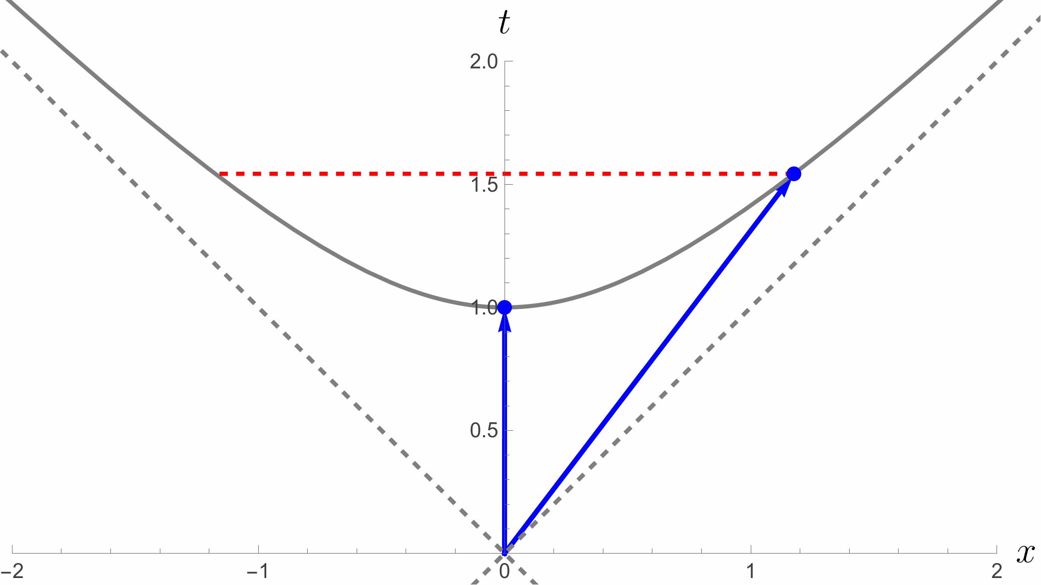
Physical interpretation is straightforward: the time interval \(d t\) is the time as measured in the rest frame of observer B, and the proper time \(d s\) is the time as measured by the moving observer A, moving at velocity \(v\) relative to B. Then
\[\tag{99} dt = \frac{ds}{\sqrt{1 - v^2}} > ds, \]
so that the stationary observer B perceives the clock of the moving observer A to be ticking more slowly. This is the well-known effect of relativistic time dilation. Figure 14 shows a spacetime diagram.
While time dilation in relativity arises from the properties of a timelike interval \(\Delta t\) under a Lorentz transformation, Lorentz contraction arises from the properties of a spacelike interval \(\Delta x\) under the same transformation. Consider a unit-length “rod’’, or a spacelike interval.
At time \(t = 0\), the rod extends from event A with coordinates \(x_A = \left(0, 0\right)\) to event B with coordinates \(x_B = \left(0, 1\right)\). Defining
\[\tag{100} \Delta x^\mu \equiv \left(x_B^\mu - x_A^\mu\right), \]
the invariant length of the rod is
\[\tag{101} \Delta s^2 = \eta_{\mu \nu} \Delta x^\mu \Delta x^\nu = -1. \]
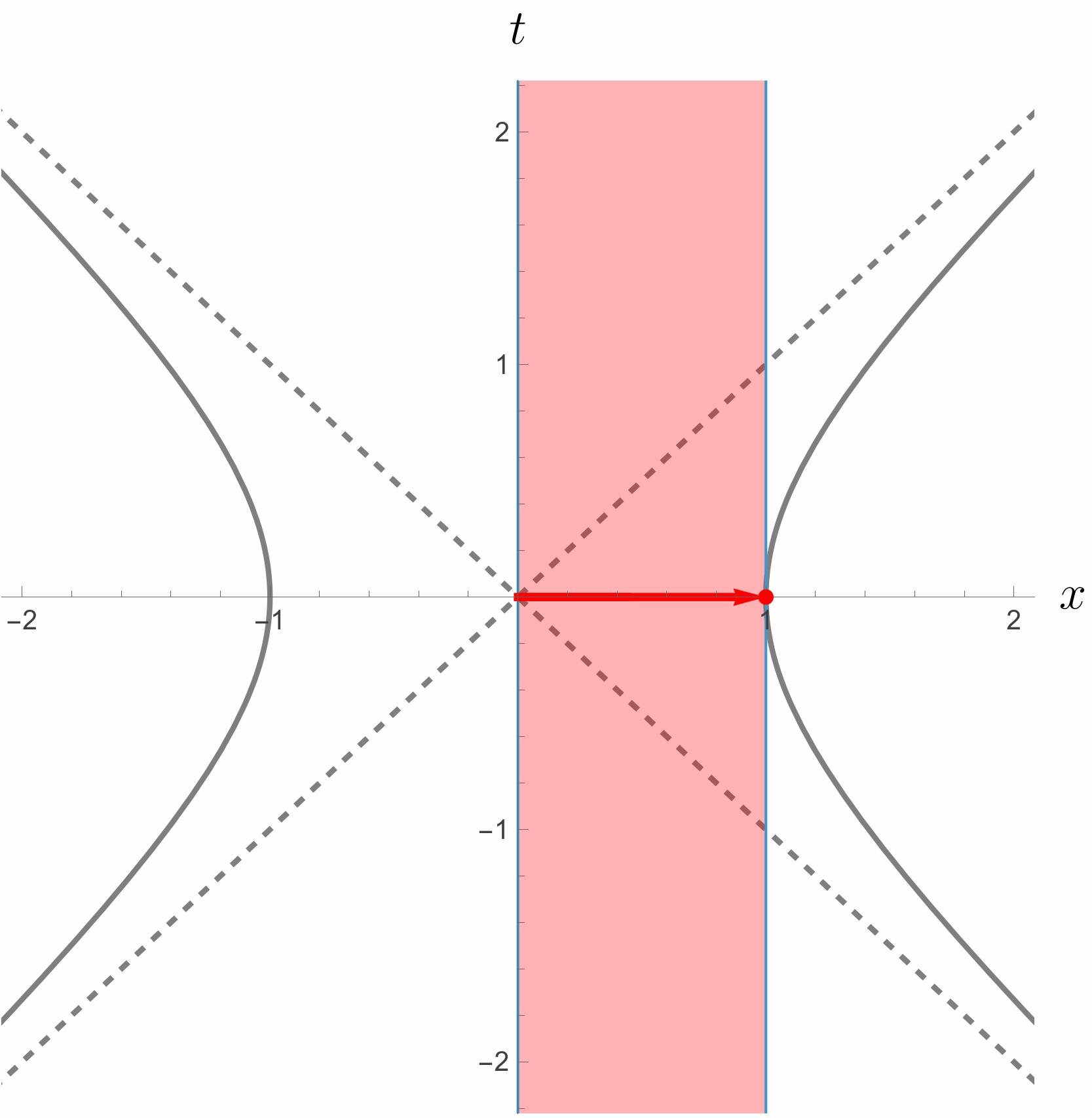
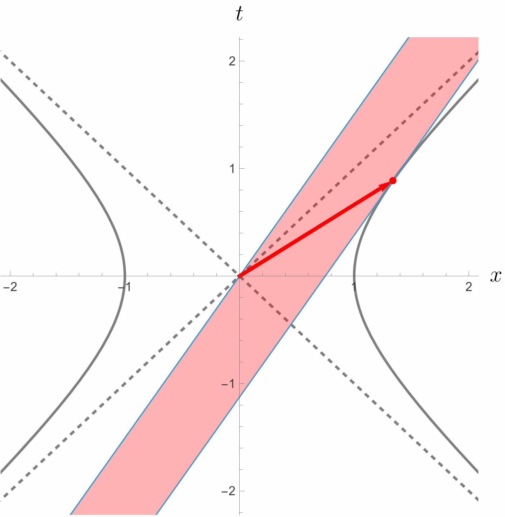
Since this is a Lorentz invariant, it is true in any inertial reference frame. Similar to a point particle tracing out a world line in time, the one-dimensional rod sweeps out a two-dimensional “world sheet’’ in time, bounded by the ends of the rod (Fig. 15). The length measured by an observer is the spatial separation between the endpoints of the rod on a hypersurface of simultaneity for that observer, for example the intersection of the rod with the \(x\)-axis at \(t = 0\). In the rest frame, the rod is of unit length.
Now consider a moving rod: the rod will Lorentz transform along the invariant hyperbola with length \(\Delta s^2 = -1\) as in Fig. 12, and the world sheet is tilted with rapidity
\[\tag{102} \xi = \tanh^{-1}\left(v\right), \]
where, \(-v\) is the relative velocity of the new rest frame, and \(v\) is the velocity of the rod. It is easy to see that the world sheet is always tangent to the invariant hyperbola: in the rest frame,
\[\tag{103} u^\mu \Delta x_\mu = 0, \]
where \(u^\mu = \left(1, 0, 0, 0\right)\) is the four-velocity, and \(\Delta x^\mu = \left(0, 1, 0, 0\right)\) is separation four-vector of the ends of the rod in the rest frame. Since this is a Lorentz-invariant quantity, it holds in any reference frame. Under a Lorentz transformation to a reference frame moving in the \(-\hat x\)-direction relative to the rod, the four-vector \(x^\mu\) transforms to
\[\tag{104} \Delta x^\mu \rightarrow \left(\Delta x'\right)^\mu = \left(\sinh{\xi},\cosh{\xi}, 0, 0\right). \]
Similarly, the four-vector \(u^\mu\) transforms at
\[\tag{105} u^\mu \rightarrow \left(u'\right)^\mu = \left(\cosh{\xi}, \sinh{\xi}, 0, 0\right). \]
Then
\[\tag{106} u^\mu x_\mu = \cosh{\xi} \sinh{\xi} - \sinh{\xi} \cosh{\xi} = 0, \]
as expected. Figure 15 shows the world sheets for the stationary and moving rod: the intersection of the world sheet of the moving rod with the \(x\)-axis (or any surface of simultaneity) has \(\Delta x < 1\), and the rod appears contracted. We can quantify the contraction by noting that the slope of the world line is just the velocity \(v = \tanh{\xi}\), so that the projected width along the \(\hat x\)-axis is
\[\tag{107} \begin{aligned} \Delta x' &= \left(\cosh{\xi} - v \sinh{\xi}\right) \Delta x\\ &= \left(\cosh{\xi} - \tanh{\xi} \sinh{\xi}\right) \Delta x\\ &= \left(\frac{\cosh^2{\xi} - \sinh^2{\xi}}{\cosh{\xi}}\right) \Delta x\\ &= \frac{\Delta x}{\cosh{\xi}} = \frac{\Delta x}{\gamma} \\ &= \Delta x \sqrt{1 - v^2}, \end{aligned} \]
recovering the usual formula for Lorentz contraction.
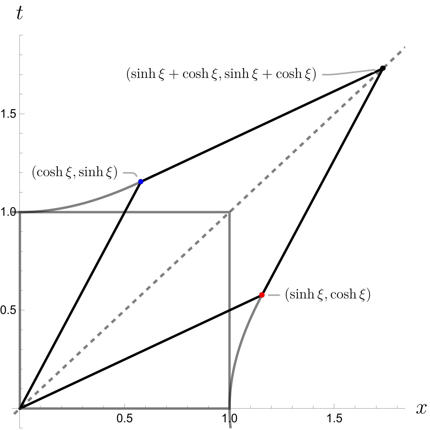
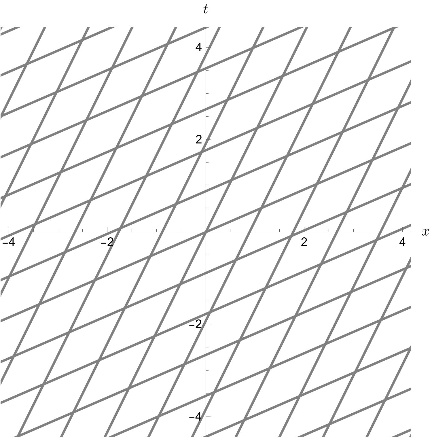
The action of the Lorentz transformation on the coordinate system can be visually summarized by the transformation of the unit square in the \(1+1\)-dimensional \(\hat x\)-\(\hat t\) plane. Figure 16 shows the Lorentz-transformation of the unit square for \(v = 0.5\): the timelike unit vector transforms along the invariant hyperbola with \(ds^2 = dt^2 - d x^2 = +1\), while the spacelike unit vector transforms along the hyperbola with \(ds^2 = -1\). The point on light cone transforms along the light cone, with \(ds^2 = 0\). Figure 17 shows the “squashing’’ of the orthogonal rest-frame coordinates into diamonds by the Lorentz transformation.
We now discuss the representation of energy and momentum as four-vector quantities. Consider a particle of mass \(m\). Since the mass m is an invariant scalar, multiplying the four-velocity by m produces another four-vector:
Definition: Four-momentum
For a particle with mass \(m\) and
four-velocity \(u^\mu\), the
four-momentum is
\[\tag{108} p^\mu \equiv m u^\mu. \]
It then follows immediately from the normalization \(u^\mu u_\mu = 1\) that the invariant magnitude of the four-momentum \(p^\mu\) is
\[\tag{109} p^\mu p_\mu = m^2. \]
The invariant hyperbola defined by \(p^\mu p_\mu = m^2\) is called the mass shell. The spatial components of the momentum four-vector are just the three-momentum \(\mathbf{p}\),
\[\tag{110} p^\mu = \left(m \frac{d t}{d s}, \mathbf{p}\right). \]
The timelike component \(p^0\) can be identified as the relativistic energy by Taylor expanding in \(v\):
\[\tag{111} \begin{aligned} p^0 &= m \frac{d t}{d s} \\ &= m \cosh{\xi} \\ &= \frac{m}{\sqrt{1 - v^2}}\\ &= m \left(1 + \frac{1}{2} v^2 + \cdots\right). \end{aligned} \]
The second term in the expansion reproduces the Newtonian kinetic energy, while the first term \(p^0 = m\) is the relativistic rest energy of the particle. Re-writing in units where \(c \neq 1\) recovers Einstein’s famous formula,
\[\tag{112} p^0 = E = m c^2 + \frac{1}{2} m v^2 + \cdots. \]
The four-momentum vector is then
\[\tag{113} p^\mu = \left(E, \mathbf{p}\right), \]
with
\[\tag{114} E = \gamma m, \quad \mathbf{p} = \gamma m \mathbf{v}. \]
The mass shell condition \(p^\mu p_\mu = m^2\) can be written in terms of the three-momentum \(\mathbf{p}\) and the rest energy \(m\) as
\[\tag{115} E^2 = \mathbf{p}{\ }^2 + m^2. \]
Just as \(x^\mu x_\mu\) is the invariant spacetime interval associated with a displacement, \(p^\mu p_\mu = m^2\) is the invariant associated with the motion of a particle.
In this section, we consider two famous paradoxes of Special Relativity, the twin paradox and the ladder/barn problem, and show how a geometric picture resolves these apparent paradoxes.
The most widely known “paradox’’ of Special Relativity is the twin paradox, in which one identical twin flies away from Earth at relativistic speed, then returns to Earth younger than the twin who remained behind, due to time dilation. The apparent paradox arises because the traveling twin should see the stationary twin’s clocks slowed by the same amount, due to the symmetry of the Lorentz transformation. The apparent paradox is easily resolved by a spacetime diagram of the problem.
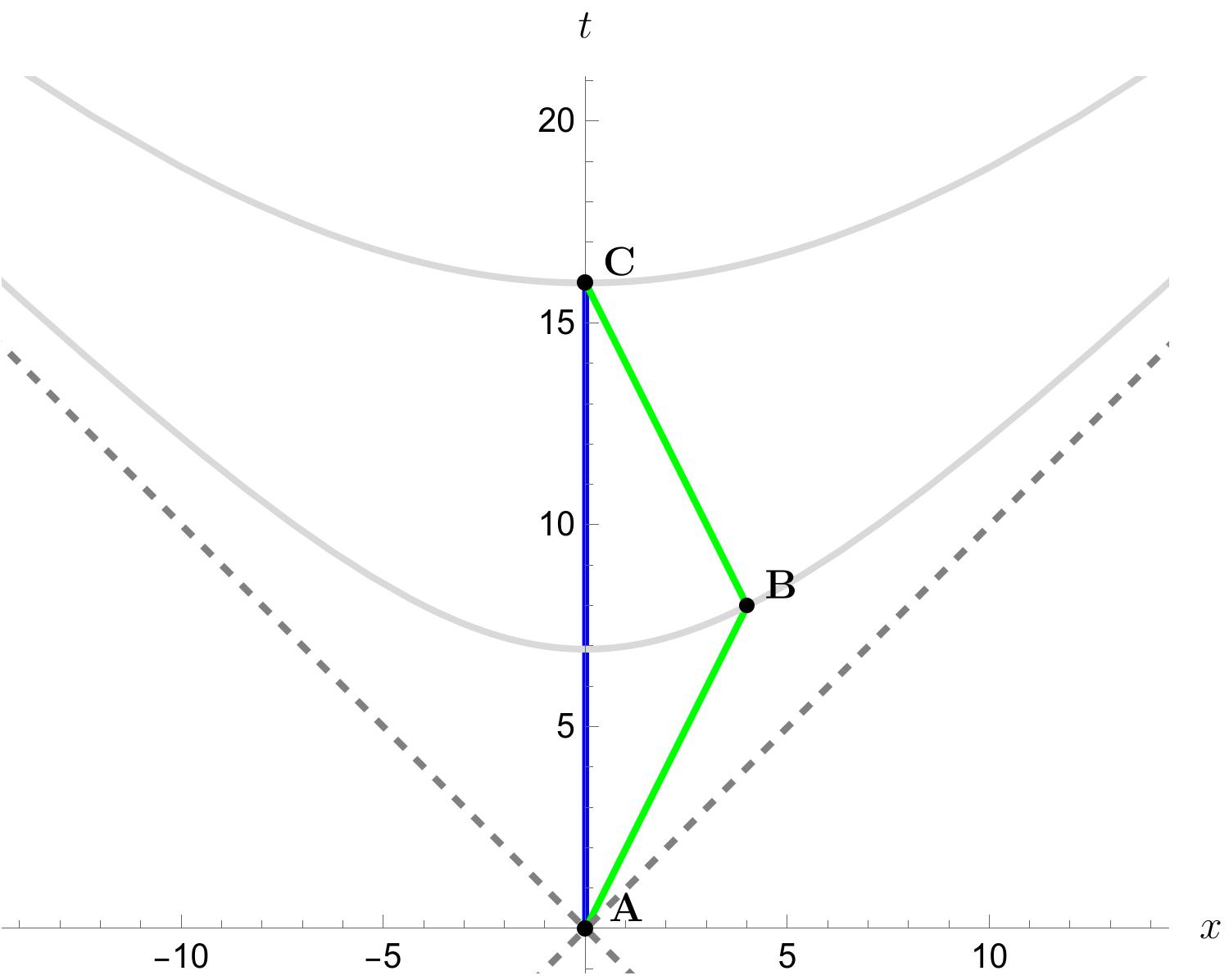
Let us suppose that the traveling twin moves at constant velocity \(v = 0.5 c\) on both the outbound and return legs of the trip, and travels 4 light years before returning. The total round-trip time in the reference frame of the stationary twin is then 16 years. Figure 18 shows the world lines of both twins in the rest frame of the stationary twin. We can calculate the round-trip time as seen by the traveling twin by calculating the proper time \(\Delta s\) along the traveling twin’s world line; just as the invariant interval between two events is independent of the observer, so is the total proper time accumulated along a world line. The coordinates of point B on the plot are \(x^\mu = \left(8, 4\right)\), so the proper time \(\Delta s\) along the outbound leg of the journey is
\[\tag{116} \begin{aligned} \Delta s^2 &= \left(\Delta t_{\text{out}}^2 - \Delta x_{\text{out}}^2\right) \\ &= \left(8^2 - 4^2\right) \\ &= 48\ \text{y}^2. \end{aligned} \]
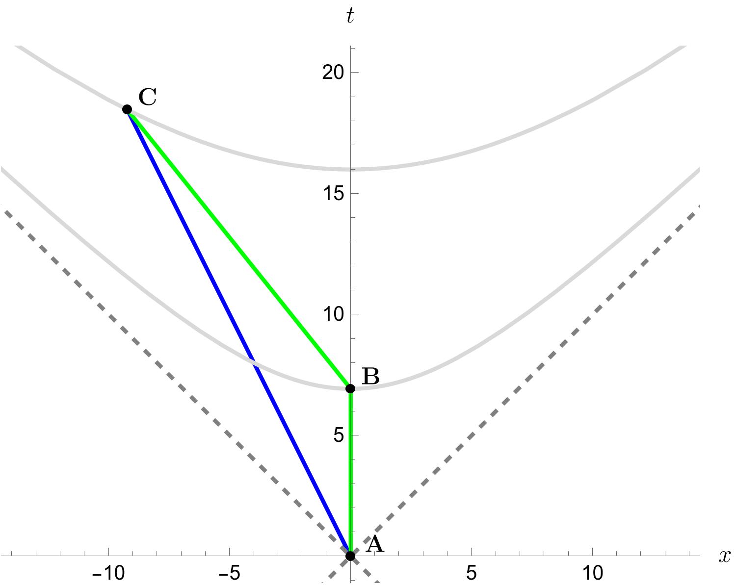
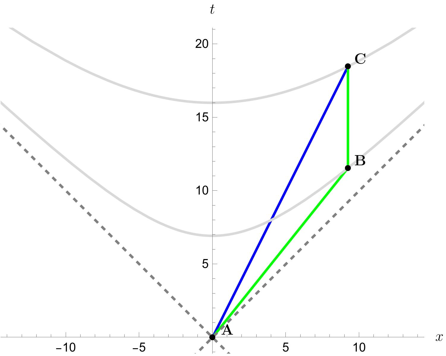
Therefore, the traveling twin measures the outbound trip to take \(\Delta s = 6.8\) years, instead of the 8 years measured by the stationary twin. By symmetry, the round trip is twice that, or 13.8 years. Because the elapsed proper time is an invariant scalar, it is valid in any reference frame. Figure 19 shows the world lines from the rest frame of the traveling twin on the outgoing leg, and from the rest frame of the traveling twin on the return leg. Events B and C on the traveling twin’s path transform along their respective invariant hyperbolae, and the proper times along the world lines are invariant. The key to resolving the apparent paradox is that there is no single reference frame in which the traveling twin is at rest the entire trip; the physical situations of the twin at rest and the traveling twin are not symmetric, and the symmetry argument for the observed time dilation fails. Note that the result follows entirely from the Lorentz-invariant proper time along the world lines, and does not rely on any effect from acceleration of the traveling twin, as is sometimes argued. This can be seen by removing the acceleration from the problem entirely: the proper time accumulated along the traveling twin’s world line would be unchanged if he continued in the same direction instead of turning around and returning to Earth.
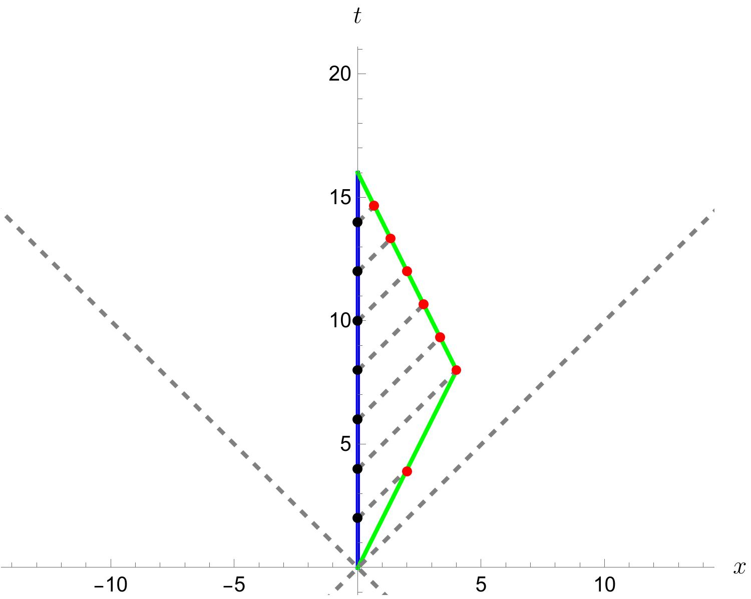
So what does the traveling twin actually see? Suppose the stationary twin carries a beacon that emits light pulses toward the traveling twin at regular intervals of proper time. Since the pulses propagate along the light cone, they take progressively longer to reach the traveling twin as he moves away from Earth. Figure 20 shows the corresponding spacetime diagram. Although the stationary twin emits the pulses at equal intervals of proper time, the traveling twin receives them at unequal intervals: the pulses arrive less frequently on the outbound leg and more frequently on the return leg. This is simply the relativistic Doppler effect: the apparent frequency of the stationary twin’s clock is redshifted on the outbound leg and blueshifted on the return leg. Both twins therefore agree that the Earthbound twin is older when they reunite.
A well-known paradox involving Lorentz contraction is the paradox of the ladder and barn. Imagine we have a 10-meter-wide barn with doors on both ends, and an 11-meter-long ladder. At rest, the ladder is too long to fit into the barn with both doors closed. However, if the ladder is moving at relativistic speed, Lorentz contraction will render the ladder short enough to fit inside the barn. The apparent paradox arises when we consider the rest frame of the ladder: in this reference frame, the barn will appear Lorentz contracted, and the ladder will again be too long to fit inside the barn with both doors closed.
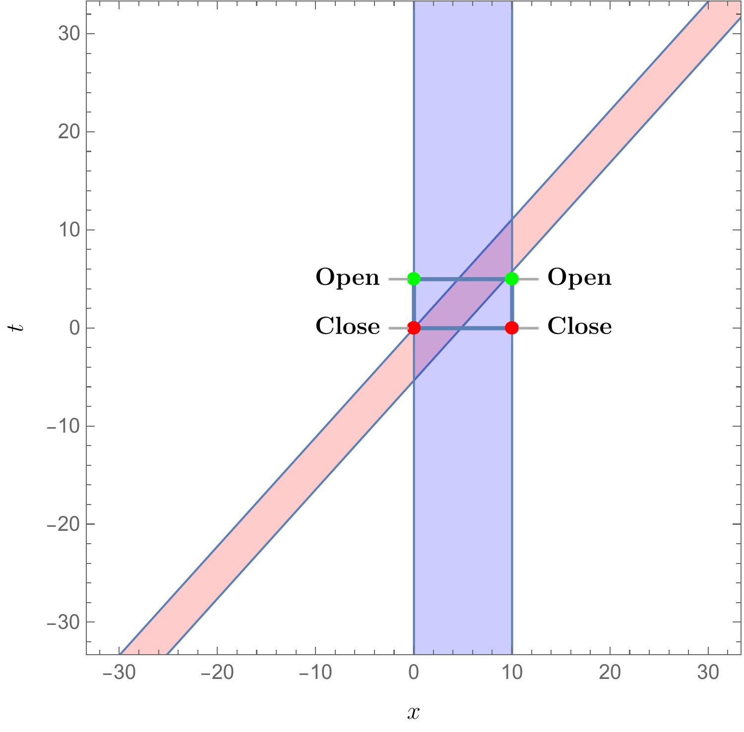
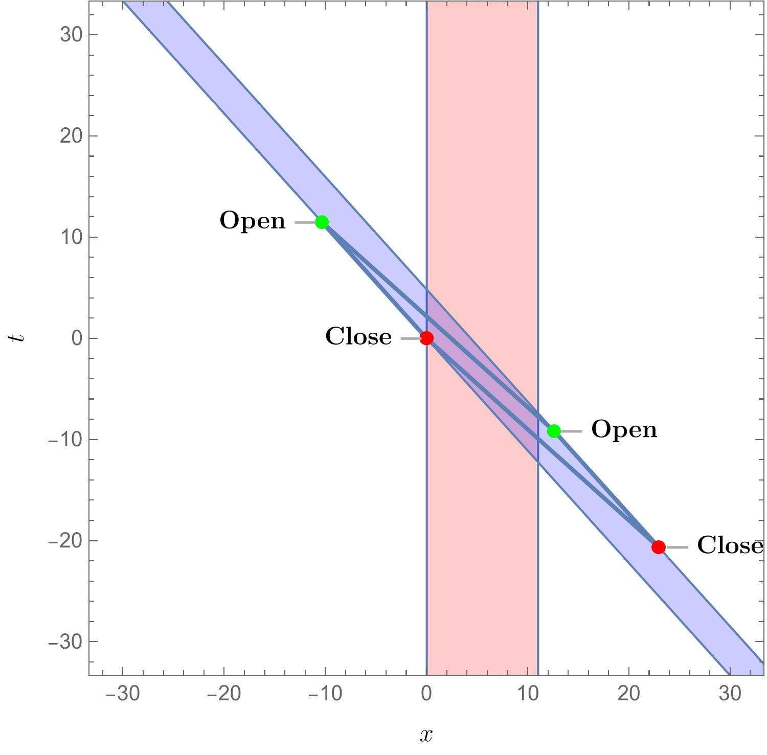
The apparent paradox is again resolved easily with a spacetime diagram. Figure 21 shows spacetime diagrams in the rest frames of the barn and ladder, respectively. The opening and closing of each barn door are spacetime events that transform independently along invariant hyperbolae. In the rest frame of the barn, the front and rear doors close simultaneously and later open simultaneously. However, because the front and rear door closing events (and likewise the opening events) are separated by spacelike intervals, their temporal ordering is not invariant. After transforming to the rest frame of the ladder, neither the closing events nor the opening events are simultaneous. In the rest frame of the ladder, the (now moving) barn passes by without the ladder colliding with the doors, but it is never inside the barn with both doors closed. Like the twin paradox, the ladder paradox is ultimately a consequence of the invariant geometry of Minkowski spacetime, in particular the relativity of simultaneity; there is no physical contradiction once the events are represented geometrically.
It is a common misconception that Special Relativity cannot be applied to accelerated reference frames, and that instead the full machinery of General Relativity is required. This is not the case! It is straightforward to handle accelerated reference frames within Special Relativity. All of the same geometric principles apply to accelerated reference frames as inertial frames, but surprising new effects arise as well, most importantly the presence of a horizon, analogous to the horizon of a black hole, when Minkowski space is observed from an accelerated reference frame, called the Rindler horizon. We begin by deriving the solution for the world line of a uniformly accelerated observer.
Consider an observer with constant acceleration relative to an local rest frame,
\[\tag{117} \mathbf{a} = \frac{d \mathbf{v}}{d t} = \text{const.} \]
As usual, we can without loss of generality confine the world line to the \({\hat t}\)-\({\hat x}\) plane, reducing the problem to \(1+1\)-dimensions,
\[\tag{118} \mathbf{a} \equiv a {\hat x} = \text{const.} \]
The four-acceleration \(a^\mu\) is then
\[\tag{119} a^\mu = \left(a^0, a, 0, 0\right). \]
Let us assume that the observer is initially at rest. In the initial rest frame, the four-velocity is
\[\tag{120} u^\mu = \left(1, 0, 0, 0\right). \]
Orthogonality then allows us to solve for the timelike component \(a^0\):
\[\tag{121} a^\mu u_\mu = - a^0 = 0\quad \Rightarrow a^0 = 0. \]
Since \(a^\mu u_\mu = 0\) is an invariant scalar, it holds in all reference frames—not just inertial frames, but non-inertial as well. We can transform to a reference frame moving with velocity \(v\) by Lorentz boosting the four-vectors \(u^\mu\) and \(a^\mu\):
\[\tag{122} u^\mu = \left(\cosh{\xi},\sinh{\xi}\right), \]
and
\[\tag{123} \begin{aligned} a^\mu &= \left(a \sinh{\xi}, a \cosh{\xi}\right) \\ &= \left(a u^1, a u^0\right) \\ &= \frac{d u^\mu}{d s}. \end{aligned} \]
Here \(s\) is the proper time along the world line of the accelerating observer. The result is a set of differential equations for the components of the four-velocity:
\[\tag{124} \begin{aligned} \frac{d u^0}{d s} &= a u^1,\\ \frac{d u^1}{d s} &= a u^0. \end{aligned} \]
If the accelerate observer is initially at rest, we have boundary conditions \(u^0\left(s = 0\right) = 1\), and \(u^1\left(s = 0\right) = 0\), with solution
\[\tag{125} \begin{aligned} u^0 &= \frac{1}{2} \left(e^{a s} + e^{- a s}\right) = \cosh{\left(a s\right)} = \frac{d x^0\left(s\right)}{d s} = \frac{d t}{d s}, \\ u^1 &= \frac{1}{2} \left(e^{a s} - e^{- a s}\right) = \sinh{\left(a s\right)} = \frac{d x^1\left(s\right)}{d s} = \frac{d x}{d s}, \\ \end{aligned} \]
where we have used the definition of the four-velocity as the derivative of the world line \(x^\mu\left(s\right)\) with respect to the proper time,
\[\tag{126} u^\mu = \frac{d x^\mu}{d s}. \]
The solution for the world line of the accelerating observer is
\[\tag{127} \begin{aligned} t\left(s\right) &= \frac{1}{a} \sinh{\left(a s\right)},\\ x\left(s\right) &= \frac{1}{a} \left[\cosh{\left(a s\right)} - 1\right], \end{aligned} \]
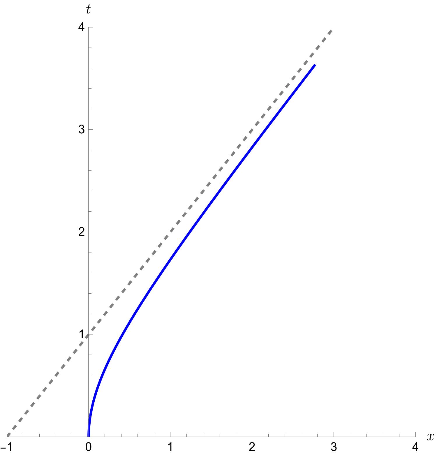
where we have fixed the integration constant by setting \(x\left(s = 0\right) = 0\). Figure 22 shows the world line \(x^\mu\left(s\right)\) for a uniformly accelerated observer. The accelerated world line asymptotes at late time to the light cone,
\[\tag{128} x \rightarrow t - \frac{1}{a}. \]
We next consider an example of uniformly accelerated motion.
Suppose we wish to travel in a rocket to the center of the Milky Way, a distance of 30,000 light years, and return to Earth. We will assume a rocket which can accelerate at a comfortable \(1\text{g} = 9.8\ \text{m} / \text{s}^2\) for half of the trip, and then decelerate at \(1\text{g}\) for the second half, and then the same for the return trip. How much time passes for an observer on the rocket? This is just the integral of the proper time along the rocket’s path:
\[\tag{129} \Delta s = \int_{x^\mu\left(s\right)}{d s}. \]
This generalizes the elapsed proper time for an inertial observer to a non-inertial observer. In both cases, the elapsed time is just the proper time measured along the world line of the observer. For our accelerated rocket, we can invert the general solution (127) so solve for \(s\left(x\right)\);
\[\tag{130} s\left(x\right) = \frac{1}{a} \cosh^{-1}\left(a x + 1\right). \]
Here we take \(x = 15,000\ \text{l y}\), representing \(1/4\) of the round trip, and then (by symmetry) multiply by four to get the total round trip time. Converting the acceleration into units where \(c = 1\) yields
\[\tag{131} \begin{aligned} \frac{a}{c} &= \frac{9.8\ \text{m} / \text{s}^2}{3 \times 10^7\ \text{m}/\text{s}} = 3.27 \times 10^{-8}\ \text{s}^{-1} \\ &= 1.03\ \text{year}^{-1}. \end{aligned} \]
It is an odd coincidence that \(1\ \text{g}\) acceleration in units where the speed of light \(c = 1\) is almost exactly one inverse year! The elapsed proper time for \(x = 1.5 \times 10^{4}\ \text{l y}\) is then
\[\tag{132} \Delta s = \frac{1}{1.03} \cosh^{-1}\left[1.03 \times \left(1.5 \times 10^{4}\right) + 1\right] = 10.04\ \text{year}, \]
a remarkably short span of time. Then the total round trip time is
\[\tag{133} \Delta s_{\text{RT}} = 40.16\ \text{year}. \]
A rocket accelerating at \(1\text{g}\) could make the round trip to the galactic center in less than a human lifetime!
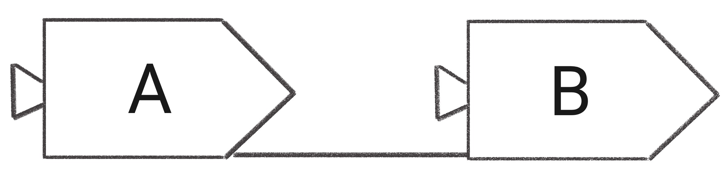
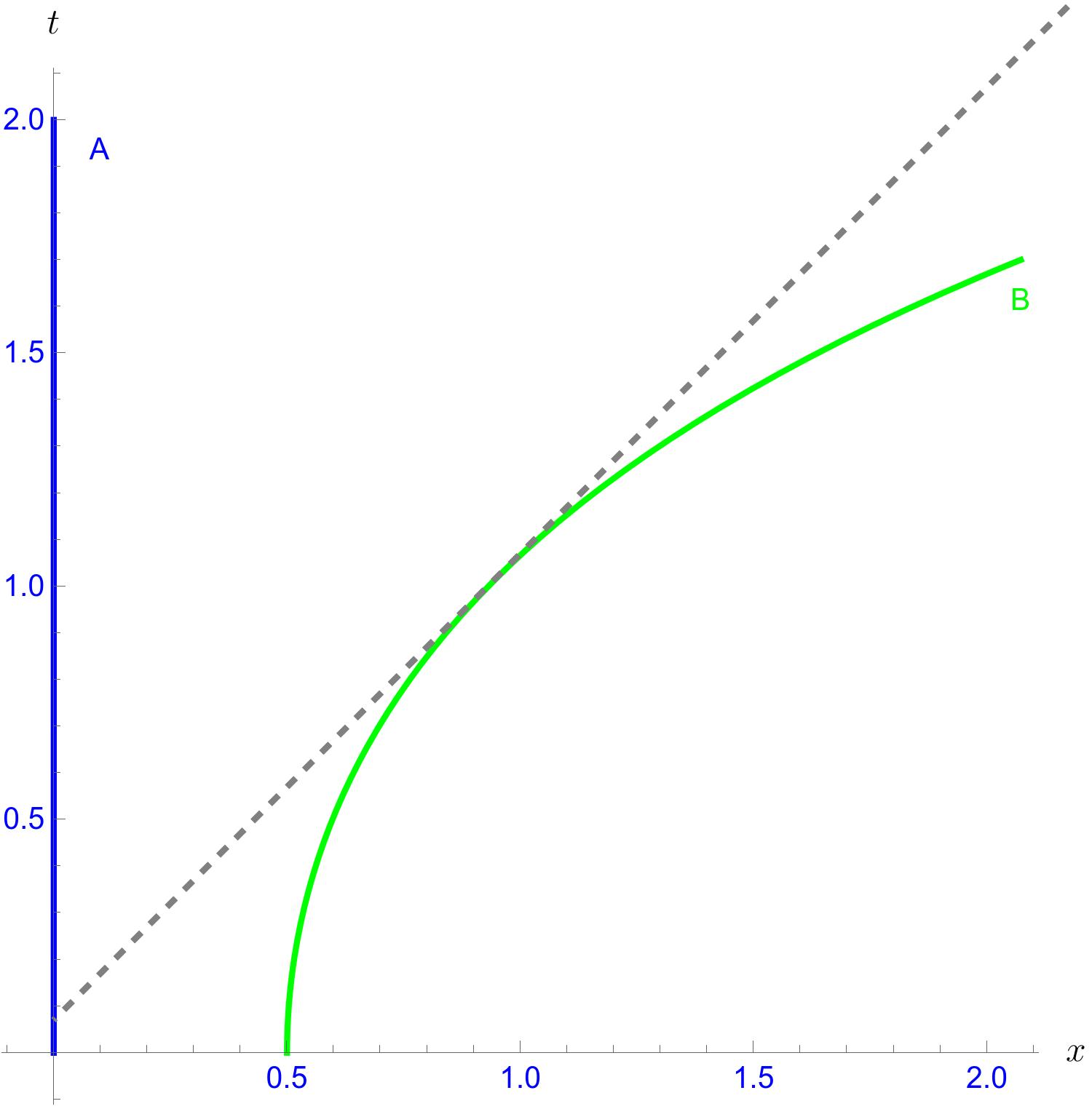
A famous problem attributed to John Bell is the problem of two identical rockets connected by a thin, breakable string (Fig. 23). The rockets are initially at rest. At time \(t = 0\), the rockets simultaneously fire (in the rest frame), and the rockets begin to uniformly accelerate, such that they maintain constant separation in the original rest frame. The world lines of the rockets then satisfy the (127), separated by a fixed distance. Figure 24 shows the world lines of the rockets in the original rest frame.
Bell’s question was this: since we expect the string to Lorentz contract as the velocities of the rockets increase, does the string therefore break, because it can no longer span the distance between the rockets? Even many very experienced physicists will (incorrectly) answer that the string will not break, reasoning that a Lorentz contraction is really just a rotation in spacetime, so the string will continue to connect the rockets in the moving reference frame. It is easy to see why this is wrong and the string breaks using a spacetime diagram (Fig. 25). Like the ladder problem, the key is again the physics of simultaneity; the Lorentz-transformed string (red arrows) connects Rocket A to Rocket B in the future, when its velocity has increased relative to Rocket A, and has therefore pulled further ahead, and the string cannot cover the gap. Rocket A’s Lorentz-transformed surfaces of simultaneity connect Rocket A to future Rocket B, with higher velocity. Similarly, Rocket B’s surfaces of simultaneity connect Rocket B to past Rocket A, with lower velocity. Although the rockets maintain constant separation in the rest frame, Rocket A sees Rocket B pulling ahead, and likewise Rocket B sees Rocket A falling behind, and observers in all three reference frames see the string break.
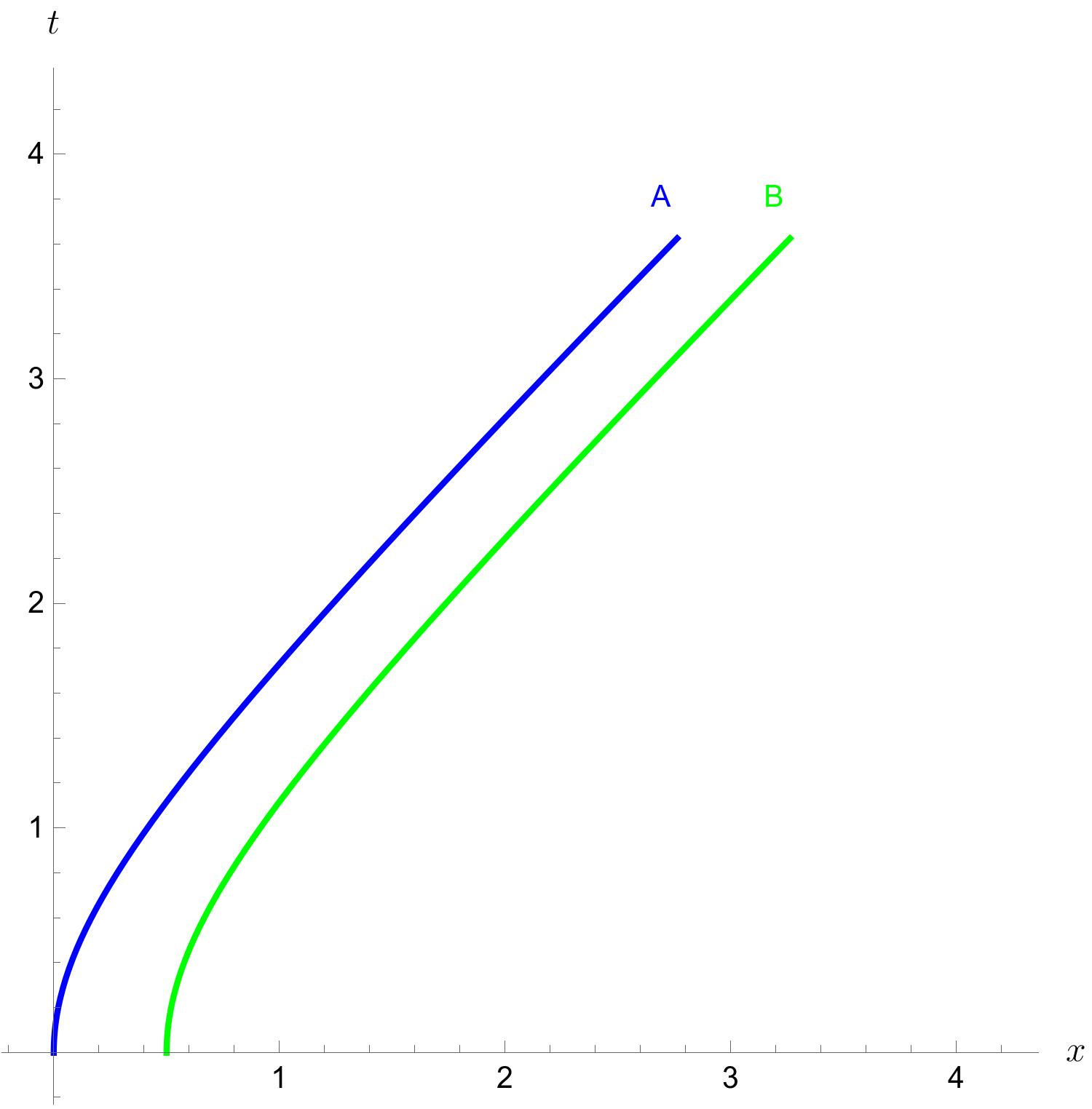
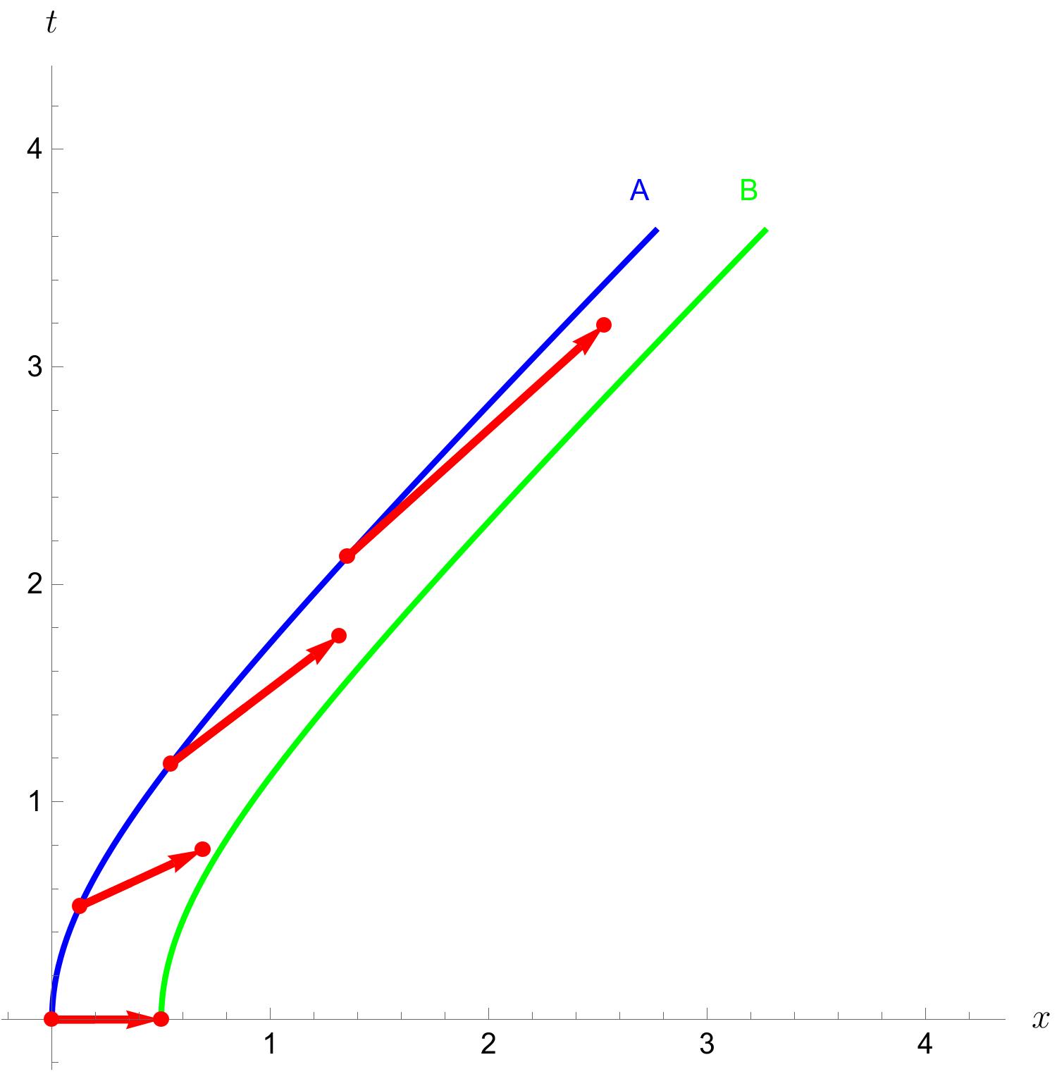
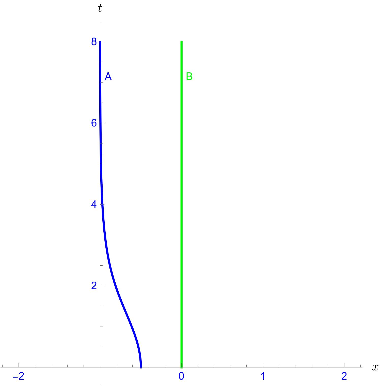
Figure 26 shows the world lines in the reference frame of Rocket A (top) and Rocket B (bottom). The results are counterintuitive: Rocket A does indeed see Rocket B pulling ahead, but (surprisingly) Rocket B eventually pulls ahead faster than the speed of light. Meanwhile, Rocket B sees Rocket A fall behind, as expected, but only for a short time, eventually coming to rest at finite distance behind Rocket B in Rocket B’s reference frame. The two observers see apparently contradictory things; this hints at a deeper structure.
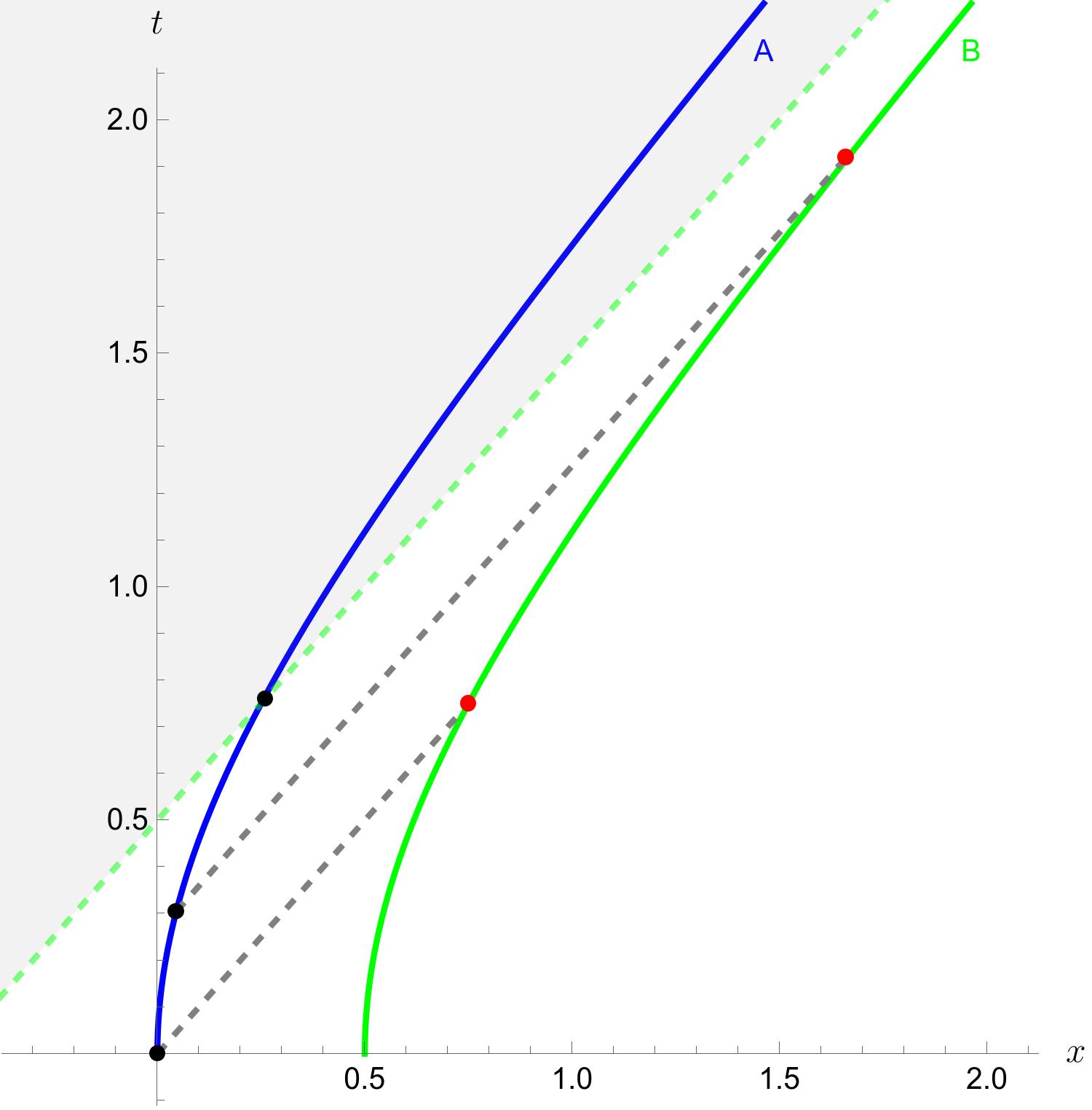
We can understand what is happening by looking at a spacetime diagram in the original rest frame of the rockets (Fig. 27). As we did for the twin paradox, let us imagine that Rocket A carries a beacon that periodically sends light pulses to Rocket B ahead; because signals travel on the light cone, it takes time for the signals to reach Rocket B, and because Rocket B is accelerating away from Rocket A, each successive signal takes longer and longer to arrive. We remember from Fig. 22 that an accelerated observer’s world line asymptotes to a light cone. Something special happens when Rocket A crosses Rocket B’s asymptotic light cone: once Rocket A is outside the light cone, any further signals sent will never arrive at Rocket B. In the rest frame (and in Rocket A’s reference frame), Rocket A passes Rocket B’s asymptotic light cone in finite time, but in Rocket B’s reference frame, it takes an infinite time. Rocket B continues to see Rocket A approaching the light cone forever, gradually slowing and coming to a stop. We interpret this as a horizon, similar to the horizon of a black hole. Just like our accelerating rockets, an observer falling into a black hole falls inside the horizon in finite time as measured by the infalling observer. But an observer outside the black hole sees the infalling observer slow down and eventually halt, taking an infinite time to fall inside the horizon. The horizon that appears in an accelerated reference frame is called the Rindler horizon, and is an artifact of the observer’s motion. Despite being an artifact, the Rindler horizon behaves very much like a black hole horizon: the space beyond the horizon is completely hidden from an observer on Rocket B. Quantum fields in an accelerated frame exhibit thermal radiation associated with the Rindler horizon. This phenomenon, known as the Unruh effect, is the flat-spacetime analog of Hawking radiation and arises because accelerating observers perceive a different quantum vacuum state from inertial observers. In general relativity it is often convenient to introduce coordinates adapted to uniformly accelerated observers, known as Rindler coordinates. These coordinates make the horizon appear explicitly in the metric, but they introduce no new physics beyond the geometric picture developed here.
An interesting twist to Bell’s original problem suggests itself: Imagine we made the string a little longer than the original gap between the ships, so that it is long enough to span the asymptotic gap between the rockets in the reference frame of Rocket B. Then Rocket A (and an observer in the rest frame) will see the string break, but the signal from the string breaking will never reach an observer on Rocket B, because no light signal emitted when the string breaks can propagate across Rocket B’s Rindler horizon. The observers therefore do not disagree about the physical event; rather, Rocket B can never obtain information about it.
I have chosen to use a mostly-minus, or “West Coast’’ metric in these notes,
\[\tag{134} \eta_{\mu \nu} = \begin{pmatrix} 1 & 0 & 0 & 0\\ 0 & -1 & 0 & 0\\ 0 & 0 & -1 & 0\\ 0 & 0 & 0 & -1 \end{pmatrix}. \]
Then the invariant interval in Minkowski space is
\[\tag{135} ds^2 = \eta_{\mu \nu} dx^\mu dx^\nu, \]
and the four-velocity has positive square norm
\[\tag{136} u^\mu u_\mu = +1. \]
An alternative (more common in the literature) is to use a mostly-plus, or “East Coast’’ metric,
\[\tag{137} \eta_{\mu \nu} = \begin{pmatrix} -1 & 0 & 0 & 0\\ 0 & 1 & 0 & 0\\ 0 & 0 & 1 & 0\\ 0 & 0 & 0 & 1 \end{pmatrix}. \]
Then the four-velocity has negative square norm,
\[\tag{138} u^\mu u_\mu = -1. \]
Conventions vary on how the proper time is defined relative to the mostly-plus metric. Most commonly, the convention is to take the invariant interval to be the same as for the opposite convention
\[\tag{139} ds^2 = \eta_{\mu \nu} dx^\mu dx^\nu, \]
and then separately define the proper time \(\tau\) as
\[\tag{140} d \tau^2 = - ds^2, \]
adding an additional (and mostly unnecessary) variable. A few fix this by retaining the proper time as the invariant interval, and defining
\[\tag{141} ds^2 = - \eta_{\mu \nu} dx^\mu dx^\nu \]
relative to the mostly-plus metric.
The choice of metric signature is purely a matter of convention—the proper time is the same in either case—but it arouses surprisingly strong opinions in many physicists, with some even declaring the mostly minus metric categorically wrong. The mostly-plus metric does have the virtue of preserving the familiar Euclidean metric for the spacelike components. It is also more convenient in field theory when defining a Wick rotation to a four-dimensional Euclidean metric to calculate certain quantum amplitudes and—depending on whom you ask—representing spinors. My goal in these notes, however, is to present Special Relativity as a geometric theory in the most direct and intuitive way possible. From that perspective, the mostly minus convention has a distinct pedagogical advantage: it is the metric convention for which vectors along physical trajectories have positive square norm. The invariant interval is most naturally interpreted as the proper time along timelike world lines, with \(ds^2 > 0\). Spacelike curves have \(ds^2 < 0\), so the proper time is imaginary, emphasizing that they cannot represent physical spacetime trajectories. Likewise, the square norm of the (timelike) four-velocity is positive, which is a more physically intuitive notion than having physical four-velocities with negative square norm.
Ultimately, the choice of metric convention is a matter of using the right tool for the job, and when looking for the simplest and most intuitive way to present a geometric picture of Minkowski space, the \(\left(+,-,-,-\right)\) metric is in my judgment clearly the superior choice. Those who disagree are entitled to a full refund on what they paid for these notes.