Dental practice is, or should be, science-based. And science runs on comparisons of groups. Thus, the reliability of assigning patients to those groups is crucial to the validity of the ensuing results. Similarly, much data are based on clinical phenomena which involve an element of judgment. So the quality of the research depends on the reliability of those data.
The basic problem is simple. You have two observers of one phenomenon. The phenomenon might be a shadow on a radiograph, a lesion in the mouth, or anything else. The two observers can be different clinicians, or could be one clinician on two occasions. How often do those two observers agree? We would like it to be always, but many clinical problems involve judgment, which can differ.
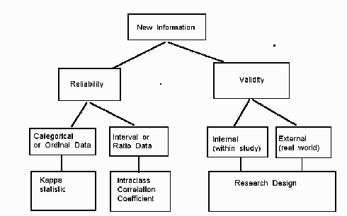
So reliability comes down to agreement, or repeatability.
Data can be classified into one of four types, and the type is important in assessing the reliability. The four types are categorical, ordinal, interval, and ratio.
Categorical data are, as the name suggests, defined by categories or classes. These categories must by mutually exclusive (that is, non-overlapping). Examples are sick or well; decayed, missing, filled, or sound. The boundaries are often arguable, which leads to the reliability question.
Ordinal data are, as the name suggests after you know it, ordered. Each category is more or less than its neighbor, but the amounts of difference between adjacent pairs may not be equal. Examples are none, mild, moderate, or severe for disease.
Interval data have equal intervals but the location of the zero is arbitrary. The classic examples are the Fahrenheit and Celsius temperature scales. The clinically important interval scales involve differences; weight loss, for example. The interval is the kilogram (or the pound for us Americans who have not caught up with the rest of the world), but the zero for weight loss is the subject's original weight.
Ratio data have equal intervals and an absolute zero. Examples of ratio data are height, weight, age. So weight is a ratio measure while weight loss (because it is a difference) is an interval measure. Notice that the fineness of the measurement does not entire into the process. Number of teeth is a ratio measure because the increments are equal (one tooth) and there is an absolute zero (no teeth).
With this background on types of data we can proceed to measurement of reliability.
For categorical and ordinal data, one uses the kappa statistic to measure reliability. For interval and ratio data, one uses the intraclass correlation coefficient (ICC).
So two observers have each observed the same subjects. For interval or ratio data, one can plot the data from one observer on one axis, the data from the other observer on the other axis, and since the two observers have each collected their data from the same subjects, each pair of observations leads to one point on the graph.
For reliable data (good agreement) we would want this plot on the graph to have three properties. First, the plot should like pretty much like a straight line without too much scatter. The amount of scatter can be quantified, but we will leave that for a statistics class. Second, the slope of that straight line should be one. If one scale (observer) says I lost 10 pounds, I sure don't want another scale saying I lost only five. And third, that straight line should go through zero. That is just another way of saying you don't want the measurements to be off by some additive amount, like having a pail of sand on one scale but not the other.
This paragraph can be skipped until after you have a statistics course. A common mistake is to use Pearson's correlation coefficient (Rp) to assess reliability of interval and ratio data. The Rp does an excellent job on the first property (amount of scatter) but fails completely on the second and third.
The intuitive idea, however, which will help you avoid the pitfalls, is fairly simple: look for the three properties given above. The calculation of the ICC involves analysis of variance and is sufficiently complicated to leave for a statistics course. The kappa statistic, in contrast, only involves some simple arithmetic.
For categorical or ordinal data each of the two observers will have counted. This many patients were positive for oral lichen planus, that many patients were negative. Or each of two observers may grade the same group of patients as mild, moderate, or severe. These sort of observations lead to a square table with the same headings on the top and the side, and the agreement goes along the main diagonal.
Here is an actual example from two oral pathologists diagnosing oral lichen planus from H & E stained slides.
| Observer 1 |
|||
| Observer 2 |
Positive for OLP |
Negative for OLP |
Row Total |
| Positive for OLP |
13 |
2 |
15 |
| Negative for OLP |
7 |
28 |
35 |
| Column Total |
20 |
30 |
50 |
The two observers agreed that 13 of the 50 patients were positive for OLP and that 28 were negative. The two observers disagreed on the other 9 patients. What are we to do with such data? An intuitive (but wrong) idea is to calculate the "percent agreement." Such a calculation leads to 26% positive and 56% negative for a total agreement of 82%. It is true that the two observers agreed on 82% of the cases, but some of that agreement was by chance. The chance probability is the product of the row probability times the column probability, as shown in Table 2.
| Observer 1 |
|||
| Observer 2 |
Positive for OLP |
Negative for OLP |
Row Total |
| Positive for OLP: Number Proportion Observed: Proportion by chance: |
13 0.26 0.12 |
2 |
15 0.30 |
| Negative for OLP: Number Proportion Observed: Proportion by chance: |
7 |
28 0.56 0.42 |
35 0.70 |
| Column Total Proportion of Total: |
20 0.40 |
30 0.60 |
50 1.0 |
The 13 cases where both observers were positive
was 0.26 of the total, but 0.12 ( = 0.4 x 0.3) was by
chance. The Kappa statistic is as follows
K = (Po
- Pc) /(1 - Pc)
where
Po is the observed proportion of
agreement,
Pc is the chance proportion of agreement,
and 1 is perfect agreement.
So both the numerator (the top)
and the denominator (the bottom) are reduced by the chance
occurrence.
In our example, Po = 0.26 + 0.56 = 0.82, and Pc = 0.12 + 0.42 =
0.54, K = (0.82 - 0.54)/(1.0 - 0.54) = 0.28/0.46 = 0.61.
So how good or how bad is 0.61 for the Kappa statistic? There are some informed (but arbitrary) guidelines:
| Kappa (K) |
Interpretation |
| K < 0.4 |
Poor |
| 0.4 ≤ K <
0.6 |
Fair |
| 0.6 ≤ K <
0.8 |
Good |
| 0.8 ≤ K |
Excellent |
See also:
http://www.emory.edu/WHSC/MED/EMAC/curriculum/diagnosis/kappa.html
http://www.ucsf.edu/~clinres/mod1/module1-3.html
http://www.human.cornell.edu/admin/statcons/Statnews/stnews31.pdf
Document revised: 09/19/03