from glob import glob
from PIL import Image
from numpy import *
import matplotlib.pyplot as pl
import os
%pylab inline

# we will compute the mean character of the images for each class
imagefolder = 'mean_character_images/'
if not os.path.exists(imagefolder):
    os.makedirs(imagefolder)


allpngs = glob('pngs/*.png')# set of all pictures names

# exctracts label for a given picture
def get_class(png): return png[-6:-4]

# list of character classes
classes = list(set([get_class(png) for png in allpngs]))
print(classes)

sampleimg = Image.open(allpngs[0])
h,w,nc = array(sampleimg).shape
Let's compute the the average image for each class
# Training step

#this line is for later
W0 = 2*np.random.random((h*w,len(classes)))


class_averages = {}# empty dictionary of form: character_class, average_image
for k,character_class in enumerate(classes):

    # list of pngs in this character_class
    pngs = [png for png in allpngs if get_class(png)==character_class]
    print(character_class,len(pngs))

    # go through all images for a given class and add together the pngs pixel-by-pixel

    average_image = zeros((h,w),dtype=float)#empty image to start

    for png in pngs:
        a = 255-array(Image.open(png))[:,:,0]  # select just the red channel (and invert)
        average_image += a

    average_image -= average_image.mean()# normalize the images by subtracting off their means

    W0[:,k] = reshape(average_image,(h*w))

    # save the mean image to a .png file
    pl.imsave(imagefolder+'average_'+character_class+'.png',average_image,vmin=average_image.min(),vmax=average_image.max(),cmap='seismic')

    # save the average_image into a dictionary
    class_averages[character_class] = average_image

#ad['_0'].max()
The shifted averages of each character class:
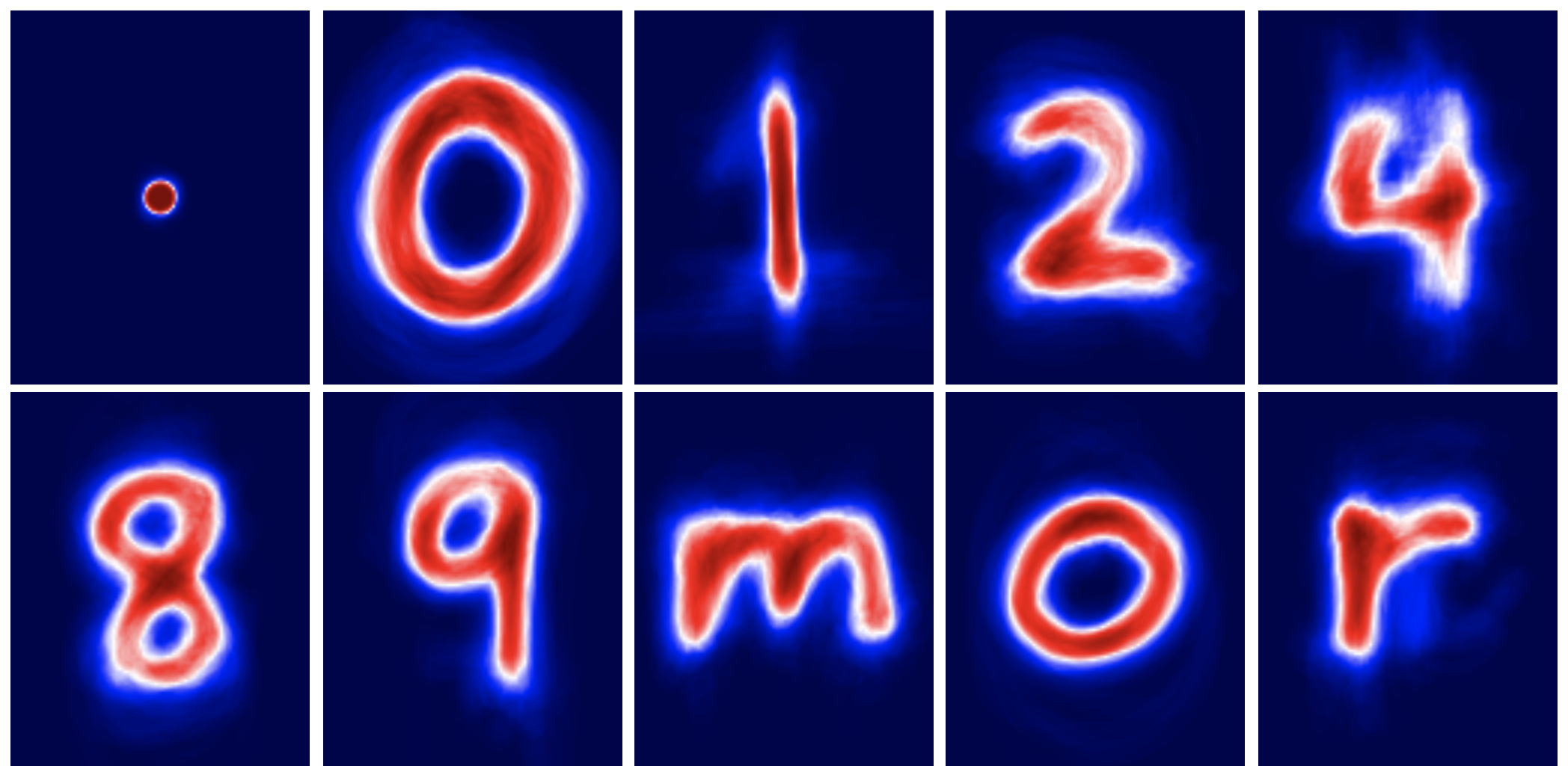
Given these averages for character recognition, we can try a simple approach to image classification:
- Compute the dot product between a given image (treating it as a vector) and the average image for each image class
- Classify each image as the the character class for which the dot product is the greatest
# testing part

for character_class in classes:

    # list of pngs in this class
    pngs = [png for png in allpngs if get_class(png)==character_class]
    #print(sig,len(pngs))

    predicted_labels = []
    for png in pngs:
        the_image = 255-array(Image.open(png))[:,:,0]  # select just the red channel (and invert)
        dot_products = []
        for class2 in classes:
            dot_products.append((the_image*class_averages[class2]).sum())# compute dot product
        predicted_label = argmax(dot_products)
        predicted_labels.append(predicted_label)
    ncorrect = sum([classes[predicted_label]==character_class for predicted_label in predicted_labels])
    print('{:2} {:4d} of {:3d}, {:2.1f}% correct'.format(character_class,ncorrect,len(pngs), ncorrect/len(pngs)*100))
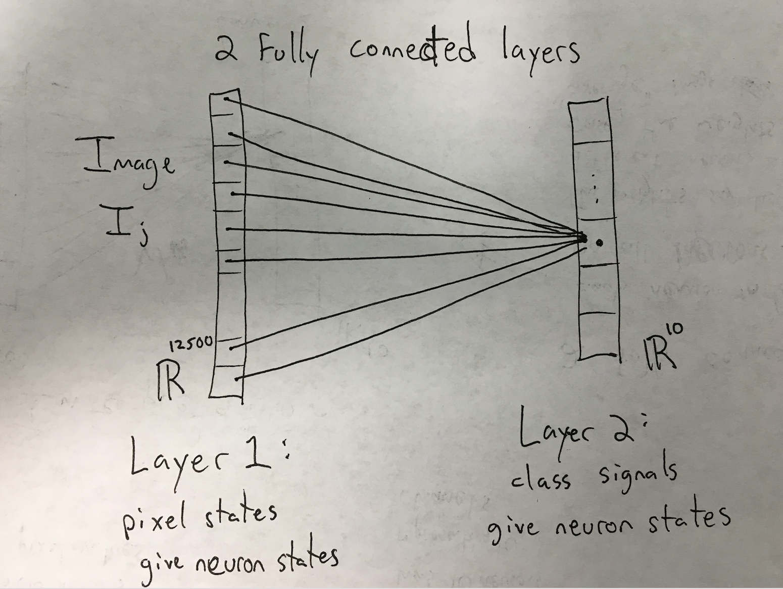
Let's now interpret this simple classifier as a neural network
For a given test image, the pixels can be interpreted as states for the 12,500 neurons in layer 1. There are 10 neurons in layer 2, and their values are interpreted as the probabilities that the image is one of the 10 classes: $\{.,0,1,2,4,8,9,m,o,r\}$. These neuron states are obtained by taking the dot product between each neurons edge weights $W$ and the states of neurons in layer 1. If, for example, the 12,500 edge weights corresponding to the first neuron in layer 1 are the mean pixel values for images of dots (see picture above), then the state of neuron 1 in layer 2 is exactly the dot product between the mean image and the test image - - exactly the same as the example from last class. Therefore, the simple linear classifier from last class can be interpreted as a neural network in which the edge weights are exactly the mean values of the images for each class.
# Construct matrix X with all training data

allpngs = glob('pngs/*.png') # set of all pictures names

n = len(allpngs)
X = zeros((n,h*w))

for i,png in enumerate(allpngs):
    a = 255-array(Image.open(png))[:,:,0]  # select just the red channel (and invert)
    X[i,:] = a.reshape((1,size(a)))

print(X.shape)
imshow(X)

# Construct matrix Y that encodes the true labels
class_dict = {}
for i,char_class in enumerate(classes):
    class_dict[char_class] = i

Y = zeros((n,len(classes)))
y_labels = zeros(n)
for i,png in enumerate(allpngs):
    #print(class_dict[get_class(png)])
    Y[i,class_dict[get_class(png)]] = 1
    y_labels[i] = class_dict[get_class(png)]

print(Y[0:20,:])
def softmax(x):
    e_x = np.exp(x - x.max())
    return e_x  / e_x.sum()

def softmax_deriv(x):
    return x*(1-x)
    #sigma = softmax(x)
    #dx = - outer(array(sigma),array(sigma))
    #dx = dx + eye(len(sigma))*sigma
    #return dx

def nonlin(x):
    X = zeros(shape(x))
    for i in range(len(x)):
        X[i,:] = softmax(x[i,:])
    return X

def nonlin_deriv(x):
    X = zeros(shape(x))
    for i in range(len(x)):
        X[i,:] = softmax_deriv(softmax(x[i,:]))
    return X
#    #return x*(1-x)
#    X = zeros(shape(x))
#    for i in range(len(x)):
#        X[i,:] = softmax_deriv(x[i,:])
#    return sum(X,axis=0)

learnRate = .1

# input dataset
#X = np.array([  [0,0,1],[0,0,1],[0,0,1],[0,0,1],[0,1,1],[1,0,1], [1,1,1]])

# output dataset
#Y = np.array([[1,0],[1,0],[1,0],[1,0],[1,0],[0,1],[0,1]])
#print(Y)

# seed random numbers to make calculation deterministic (just a good practice)
np.random.seed(1)

# initialize weights randomly with mean 0
W0 = 2*np.random.random((shape(X)[1],shape(Y)[1]))
W0 = W0 - mean(W0)
#W0

for iter in range(1000):

    # forward propagation
    l0 = X
    l1_i = np.dot(l0,W0)
    l1 = nonlin(l1_i)

    # how much did we miss?
    l1_error = Y - l1
    cost = .5 * sum(l1_error**2)
    #print(l1_error)
    #print(cost)

    # multiply how much we missed by the true labels

    #print(shape(l1_error))
    #print(shape(nonlin_deriv(l1)))

    l1_delta = learnRate * l1_error * nonlin_deriv(l1)

    shape(l1_delta)
    # update weights
    W0 += learnRate * np.dot(l0.T,l1_delta)
    #break

    l1_argmax = argmax(l1,axis=1)
    Y_argmax = argmax(Y,axis=1)
    print(sum(Y_argmax!=l1_argmax))
print("Output After Training:")
print(l1)
print(Y)
l1_argmax = argmax(l1,axis=1)
Y_argmax = argmax(Y,axis=1)
print(sum(Y_argmax!=l1_argmax))

scatter(Y_argmax,l1_argmax)
np.savetxt('true_vs_predicted_labels.csv', ([l1_argmax.T,Y_argmax.T]), delimiter=',',fmt='%d')

Only 1 out of 2286 images is incorrectly classified!
Wait a second.... Recall that we are training and testing on the same dataset. Thus, 99.99% correct classification is not that unexpected. We will find errors if we split the data into testing and training data and then implement cross validation.
Let's have a look at the final weight matrices
# we will compute the mean character of the images for each class
imagefolder2 = 'neural_network_weight_images/'
if not os.path.exists(imagefolder2):
    os.makedirs(imagefolder2)

for k in range(shape(W0)[1]):
    character_class = classes[k]
    weight_image = reshape(W0[:,k],(h,w))
    imshow(weight_image)
    pl.imsave(imagefolder2+'weight_matrix_'+character_class+'.png',weight_image,vmin=weight_image.min(),vmax=weight_image.max(),cmap='seismic')
