Support Vector Machines (SVM)

The Perceptron Learning Algorithm (PLA) identifies a plane $W$ that separates linearly separable data. The algorithm converges (i.e., stops) when such a plane is found. It does NOT seek to find the BEST plane.

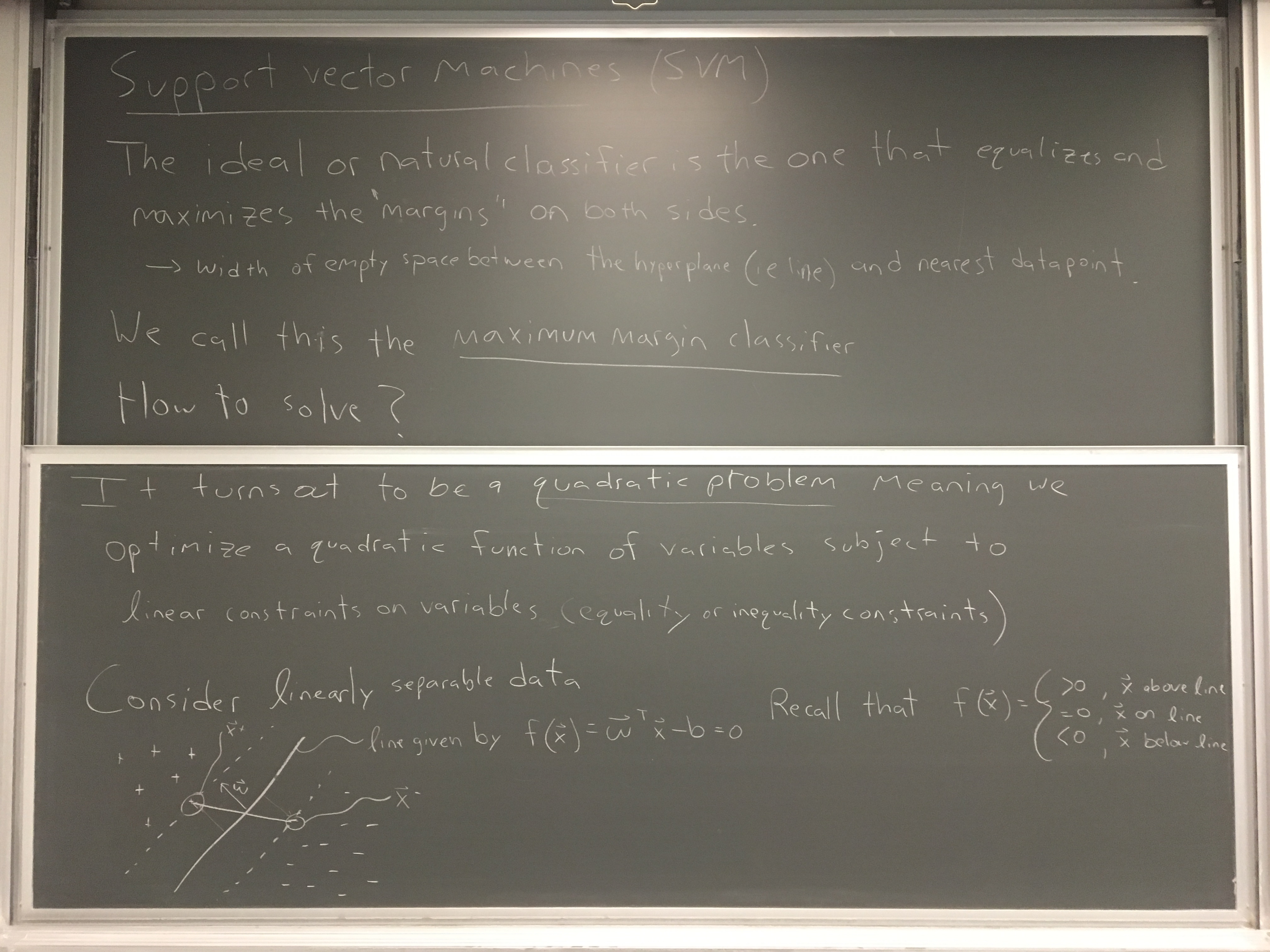
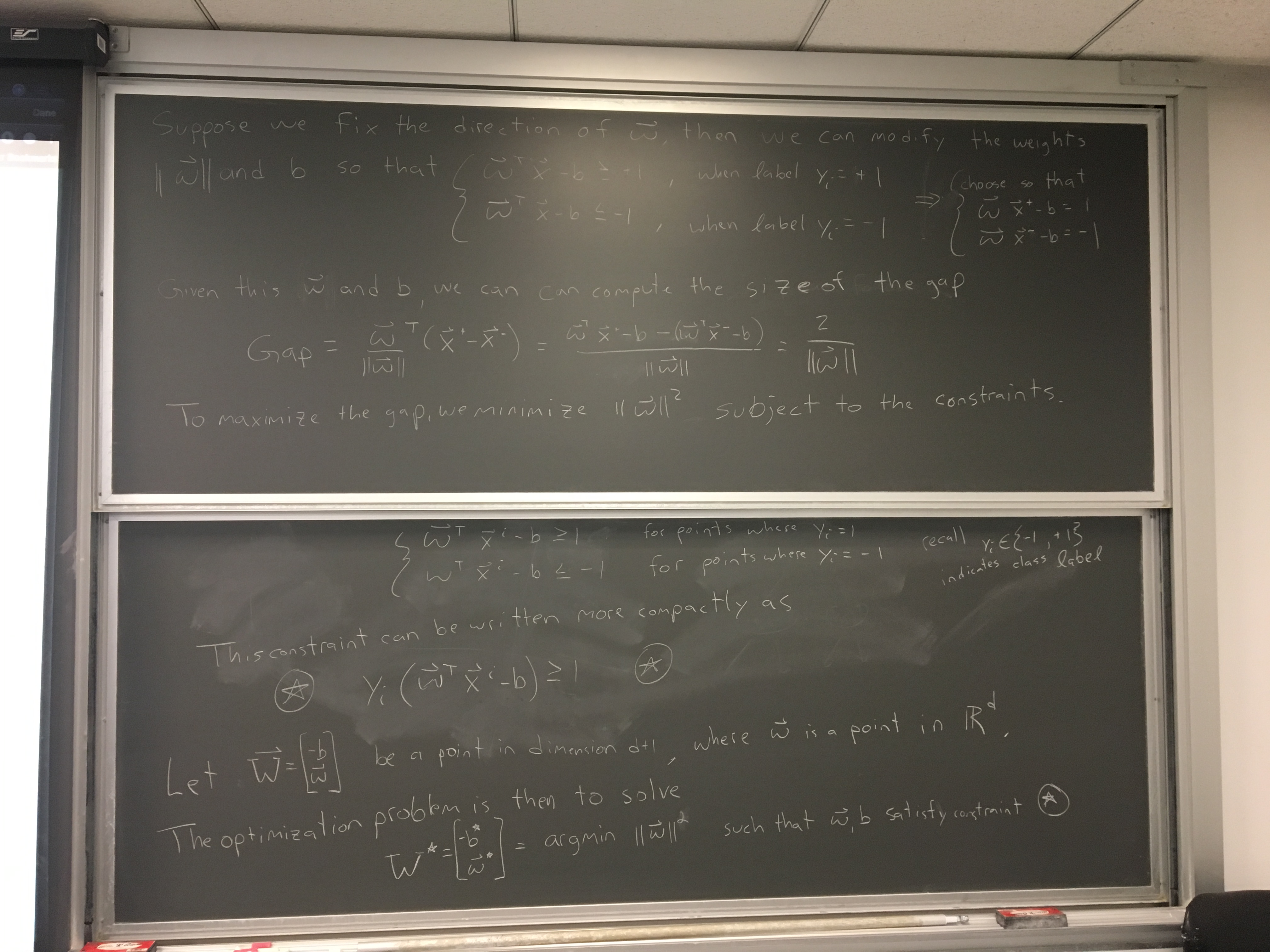
To this end, we study support vector machines (SVMs). SVMs aim to find the maximum margin classifier as the solution of a quadratic programming problem. The approach involves 2 steps:

  1. Formulate the BEST plane as a convex optimizaiton problem
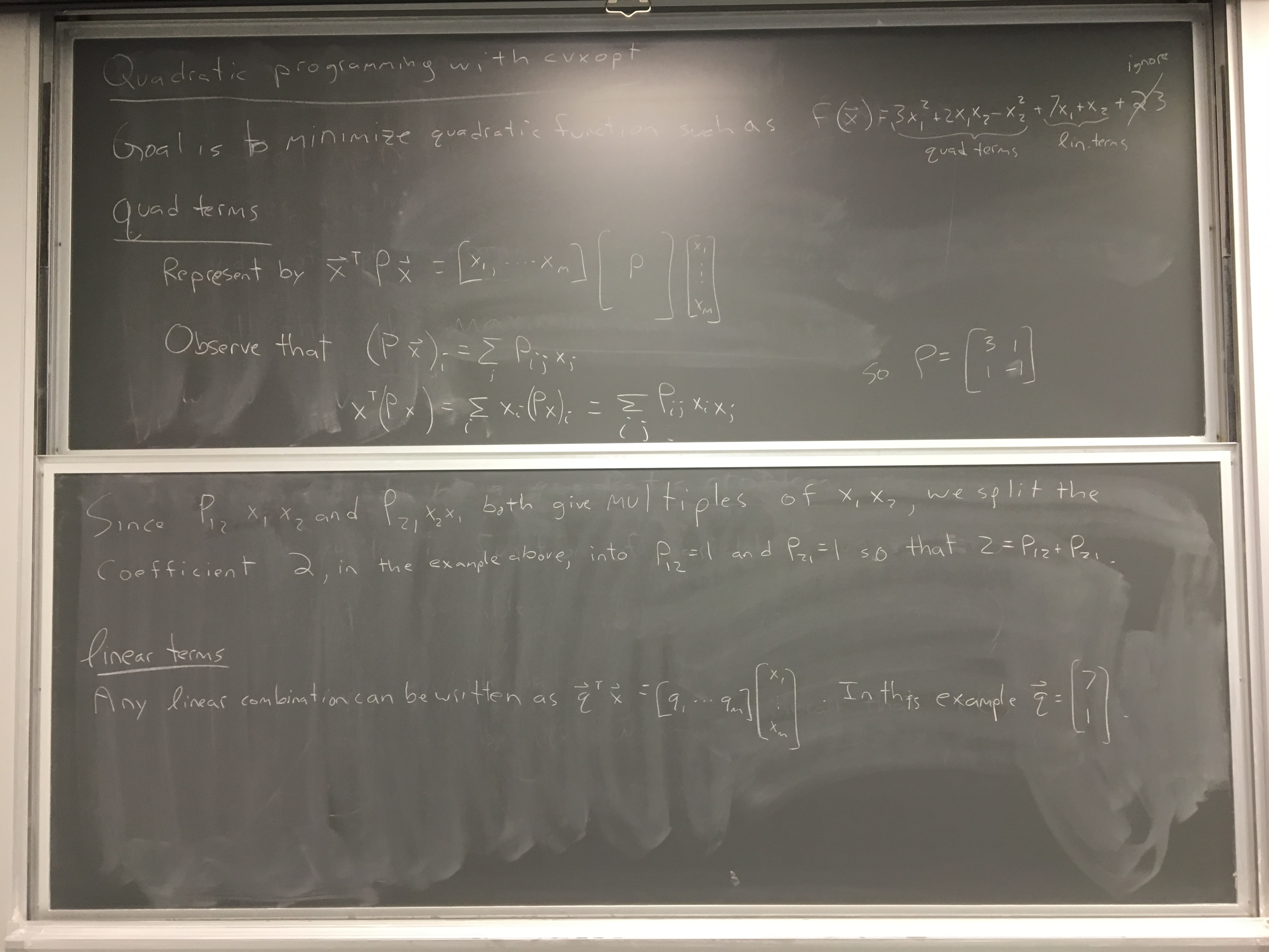
  2. Solve the convex optimization problem using quadratic programming

Below are the notes from class

Let's first cook up some linearly separable data to study

In [6]:
def create_data(n,d):
    x = random.rand(d,n) #randomly place points in 2D
    X = empty((d+1,n))
    X[0,:] = 1
    X[1:,:] = x    
    y = sign(dot(W_true,X))  
    halfgap = 0.05
    X[-1,y>0] += halfgap
    X[-1,y<0] -= halfgap
    return X,y
In [7]:
from numpy import *
d = 2 #2 dimensions
n = 50 #data points
W_true = array([-1,-2,3.])  # the true separating line (adding dot forces array to be a float array)
X,y = create_data(n,d);

#print(x)
print(X)
#print(y)
[[  1.00000000e+00   1.00000000e+00   1.00000000e+00   1.00000000e+00
    1.00000000e+00   1.00000000e+00   1.00000000e+00   1.00000000e+00
    1.00000000e+00   1.00000000e+00   1.00000000e+00   1.00000000e+00
    1.00000000e+00   1.00000000e+00   1.00000000e+00   1.00000000e+00
    1.00000000e+00   1.00000000e+00   1.00000000e+00   1.00000000e+00
    1.00000000e+00   1.00000000e+00   1.00000000e+00   1.00000000e+00
    1.00000000e+00   1.00000000e+00   1.00000000e+00   1.00000000e+00
    1.00000000e+00   1.00000000e+00   1.00000000e+00   1.00000000e+00
    1.00000000e+00   1.00000000e+00   1.00000000e+00   1.00000000e+00
    1.00000000e+00   1.00000000e+00   1.00000000e+00   1.00000000e+00
    1.00000000e+00   1.00000000e+00   1.00000000e+00   1.00000000e+00
    1.00000000e+00   1.00000000e+00   1.00000000e+00   1.00000000e+00
    1.00000000e+00   1.00000000e+00]
 [  8.59534323e-01   9.73868901e-01   4.22565158e-01   4.49185703e-01
    8.46685032e-01   3.95790512e-01   5.25241900e-01   4.47601179e-01
    1.41833277e-01   7.95049405e-01   9.16595861e-01   2.31353990e-01
    4.49664777e-01   5.59550315e-01   2.52767595e-01   1.56882628e-01
    4.85880814e-01   1.46914247e-01   8.21899122e-01   1.46203788e-01
    4.43141186e-01   1.39592961e-01   2.52384202e-01   2.15540125e-01
    9.10828948e-01   9.82112823e-01   6.54595053e-01   7.09381992e-01
    1.44595566e-01   1.53130244e-02   6.83083272e-01   2.85564867e-01
    1.53485838e-01   3.37417094e-01   9.41938462e-02   3.79163584e-01
    2.34299136e-01   1.84241922e-01   4.60855581e-01   3.11596017e-01
    1.07936712e-01   9.20700427e-01   2.72487619e-01   6.66280156e-01
    7.49289997e-01   1.39411625e-01   8.75817481e-01   8.49896999e-02
    9.28285169e-01   4.66631374e-01]
 [  4.34114839e-01   6.55518342e-01   8.42333413e-01   7.96260913e-01
    9.14748775e-03   8.55322983e-01   1.55919365e-01   9.82782569e-01
    8.89181435e-02   2.64249916e-01   2.18174161e-01   6.20564638e-01
    8.54780049e-01   5.92998115e-01   8.26039856e-01   4.71551701e-02
    4.01514955e-01   7.19871244e-01   1.00745003e+00   4.62669265e-02
    9.86742721e-01   9.49516297e-01   2.82905667e-01   9.83248938e-01
   -8.25364748e-03   4.01063664e-01   9.00643031e-01   2.67915876e-01
    9.09415075e-01   7.60520156e-01  -6.74953126e-04   8.63005483e-01
    5.98718683e-01   3.04976507e-01   4.55393151e-02   9.43563707e-01
    8.83138375e-01   3.37564868e-01   8.34449033e-01   1.50278928e-01
    2.22554734e-01   3.94889785e-01   1.00540876e-01   5.09217326e-01
    6.82208860e-01   1.78405713e-03   6.70030709e-01   8.13172805e-01
    5.68538237e-01   4.82367255e-01]]

Create some functions to plot the data

In [8]:
def draw_points(X,y):
    subplot(111,aspect=1)
    xp = X[1:,y>0]
    xm = X[1:,y<0] 
    plot(xp[0],xp[1],'rx')
    plot(xm[0],xm[1],'bx');
    
def drawline(W,color='g',alpha=1.):
    plot([0,1],[-W[0]/W[2],-(W[0]+W[1])/W[2]],color=color,alpha=alpha)

Now let's plot the data

In [9]:
%pylab inline
draw_points(X,y)
drawline(W_true,color='c',alpha=.5)
Populating the interactive namespace from numpy and matplotlib

Prepare the parameters for cvxopt solver

See notes

Note: You will need to install cvxopt. Google "conda install -c anaconda cvxopt"

In [10]:
from cvxopt import matrix,solvers
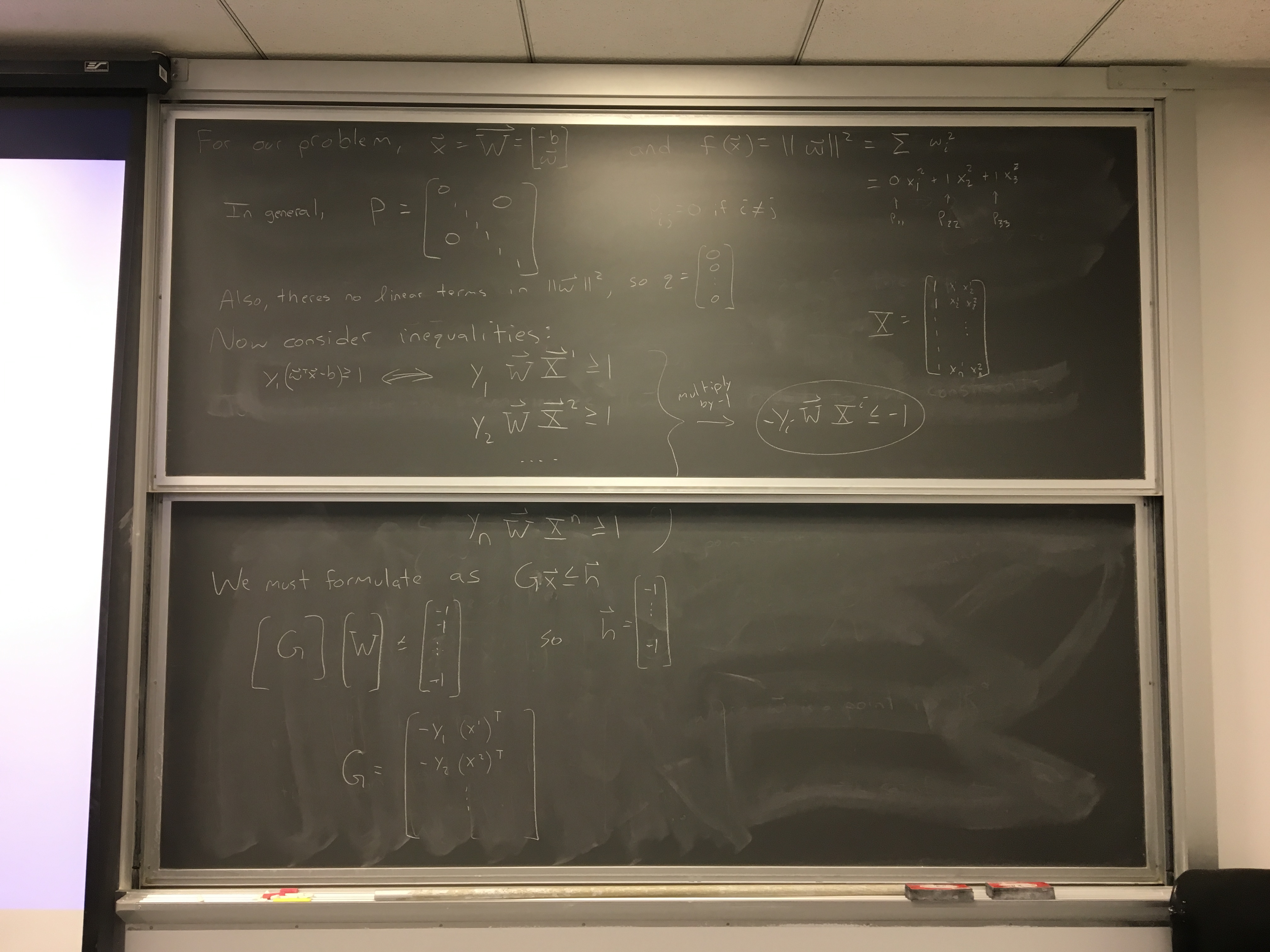
P = eye(d+1)
P[0,0] = 0
q = zeros(d+1)
G = (-X*y).T
h = -ones(n)

P = matrix(P)
q = matrix(q)
G = matrix(G)
h = matrix(h)

Solve the problem

In [11]:
sol=solvers.qp(P,q,G,h)
     pcost       dcost       gap    pres   dres
 0:  2.5019e+00  3.8657e+01  2e+02  2e+00  3e+01
 1:  1.7660e+01  3.4407e+00  4e+01  5e-01  6e+00
 2:  2.1629e+01  9.9967e+00  4e+01  4e-01  6e+00
 3:  3.9385e+01  3.5251e+01  2e+01  2e-01  2e+00
 4:  4.8428e+01  4.7684e+01  1e+00  4e-03  5e-02
 5:  4.8575e+01  4.8560e+01  2e-02  4e-05  5e-04
 6:  4.8576e+01  4.8575e+01  2e-04  4e-07  5e-06
 7:  4.8576e+01  4.8576e+01  2e-06  4e-09  5e-08
Optimal solution found.
In [12]:
type(sol)
Out[12]:
dict
In [13]:
sol.keys()
Out[13]:
dict_keys(['x', 'y', 's', 'z', 'status', 'gap', 'relative gap', 'primal objective', 'dual objective', 'primal infeasibility', 'dual infeasibility', 'primal slack', 'dual slack', 'iterations'])
In [14]:
W = array(sol['x']).reshape(d+1)
print(W)
[-2.86676308 -5.40140402  8.24474863]

Plot the solution

In [15]:
draw_points(X,y)
drawline(W_true,color='c')
drawline(W,color='k')

Here is a second implementation that uses quadprog rather than cvxopt

In [43]:
import quadprog 
def quadprog_solve_qp(P, q, G=None, h=None, A=None, b=None):
    qp_G = .5 * (P + P.T)   # make sure P is symmetric
    qp_a = -q
    if A is not None:
        qp_C = -numpy.vstack([A, G]).T
        qp_b = -numpy.hstack([b, h])
        meq = A.shape[0]
    else:  # no equality constraint
        qp_C = -G.T
        qp_b = -h
        meq = 0
    return quadprog.solve_qp(qp_G, qp_a, qp_C, qp_b, meq)[0]
In [44]:
P = eye(d+1)
P[0,0] = .000000001
q = zeros(d+1)
G = (-X*y).T
#print(G)
h = -ones(n)
W2 = quadprog_solve_qp(P, q, G, h, A=None, b=None)
print(W2)
[-2.86676308 -5.40140402  8.24474864]
In [47]:
draw_points(X,y)
drawline(W_true,color='c')
drawline(W2,color='k')

SAME ANSWER

Exercise 1

Repeat homework 4 (cross validation) for the SVM and compare your results to the PLA.

Exercise 2

Consider 2-dimensional data with 4 class labels separated by 2 hyperplanes (visualize an x splitting the unit square into 4 domains). Modify the SVM algorithm to implement a decision tree that first separates according to one hyperplane and then according to the other.