1. Getting Started
1. Create a new folder called MTH309_NumpyLabs
2. Save the file http://www.acsu.buffalo.edu/~danet/Sp18/MTH309/MTH309_files/NumpyLab1.zip into that folder and uncompress the '.zip' file
* The file NumpyLab1.ipynb is a template for today's lab
* The file mth309.py is a resource file that has specialized functions for our class!
3. Open file 'NumpyLab1.ipynb'
* On a mac, navigate to the folder called NumpyLab1 using the 'cd' command in your terminal application
* When in the correct folder using the terminal application, type: jupyter notebook NumpyLab1.ipynb
* This should launch a jupyter notebook in your web browser
2. Intro to Anaconda, Python and Numpy
Python is a programming language. It is similar to Matlab and R. It is not as low-level as c or c++. It is probably the most widely used programming language for data science and computer science.
Anaconda is a software distribution manager. It is used to install and update software including python itself and python modules, such as NumPy. Installation and update is implemented using conda
* For example, in a terminal write: 'conda update python'
Numpy [num-pie = numerical + python] is a python module designed for linear algebra.
# First thing, you must import the numpy module.

from numpy import *

# Also, did you notice that anything written after '#' is commented out.
# Write comments. Write lots of comments.
Creating arrays
Numpy arrays can be created from lists of numbers, or lists of lists of numbers, using numpy's array function.
Lists in python are comma-separated sequences of things enclosed by square brackets, like this: [2,4,6,8].
Note that Jupyter Notebook automatically prints the value of the last expression in a cell, but you need to explicitly "print" anything else you want to see. You can also "print" the last expression in a cell, and for a numpy array that gives a cleaner rendering.
x = array([1,20,300])
x
print(x)
print('This is something')
print(10*x)
A two-dimensional numpy array, which we will use as a matrix in this course, can be constructed from a list of its rows:
a = array( [[1,2,-3], [7,8,4]] )
print(a)
There are functions in numpy to create frequently-used special matrices such as the "identity" matrices and zero matrices.
print(eye(3))
#print(5*eye(3))
zeros(3)
zeros((2,5))
You can make random matrices that contain integers using random.randint
A = random.randint(0,10,(3,9))
print(A)
a = array( [[1,20,-300], [7,80,900]] )
print(a)
print(a[0][0])
print(a[0])
print(a[1])
print(a[1][:2])
Arithmetic on arrays¶¶
u = array([1,2,3])
v = array([0,10,100])
print(u)
print(v)
Numpy allows us to do arithmetic on arrays very easily.
To add the two arrays above elementwise, as in vector addition, we just write u+v as you'd expect:
print(u+v)
We can also do scalar multiplication easily:
print(u + 100*v)
There are 2 ways to change a variable
u = u*10;
v *= 10; # you can also write +=, -=, /=,
print(u)
print(v)
3. Linear Algebra with Numpy
Let's consider (modified) Exercise 13 from Chapter 1.2, which asks us to find the general solution for a system whose augmented matrix is given by
We will solve it 2 ways:
- Using Numpy arrays and row reductions
- Using the rre function from mth309.py
First approach: Using Numpy arrays and row reductions
#first define the augmented matrix encoding the system of equations

a = array([[ 1,-3, 0,-1, 0,-2],
           [ 0, 1, 0, 0,-4, 1],
           [ 0, 0, 0, 0, 0, 0],
           [ 0, 0, 0, 1, 9, 4]],dtype=float)
print(a)
Step 1: Swap row 3 and row 4.
Note that because counting starts at 0,1,2, ... in python, these rows 3 and 4 are indexed 2 and 3.
a[[2,3]] = a[[3,2]]
print(a)
Step 2: Cancel out the -3 in row 1. (i.e., row 0)
a[0] = a[0] + 3*a[1]
print(a)
Step 3: Cancel out the -1 in row 1. (i.e., row 0)
a[0] = a[0] + a[2]
row_echelon_form = a;
print(row_echelon_form)
The matrix is now in reduced echelon form!
Second approach: Using the 'rre' function from mth309.py
# first load mth309
from mth309 import *

print(a)

print('\n Using the rre function, we can obtain the reduced echelon form with 1 line of code!')
print(rre(a))
Using the function 'Matrix' from
The function matrix allows rational fractions to be depicted as fractions and not decimals.
#Lets create a random matrix

random.seed(777) # This line is just to ensure that the following "random" matrix is the same every time you execute this cell
A = random.randint(0,10,(3,4))
print(A)
a = Matrix(A)  # create an array whose elements are rational numbers (actually fractions.Fraction)
print(a)
print(a/2)
print(A/2)
Let's compute the row-reduced echelon form of A
print(rre(a))
print(rre(A))
We can compare with the result from the built-in (floating-point) linear solver linalg.solve(). First let's convert our answer to approximate decimal form:
linalg.solve(A[:,:3],A[:,3])
To convert the fractions back to decimals, use the function decimalized
decimalized(rre(A))
Agreement!
4. Applications from Ch. 10.6
Application 1: Balancing Chemical Equations (see page 52 in book)
Balance the following chemical equation:
Note that:
- $C_3H_8$ is propane
- $O_2$ is oxygen
- C0_2 is carbon dioxide
- $H_20$ is water
Balancing the equation means that the carbons, hydrogens and oxygens must be conserved. We set the system up using vectors:
- row 1 encodes carbon conservation
- row 2 encodes hydrogen conservation
- row 3 encodes oxygen conservation
Thus this system is equivalent to:
Step 1 is rewrite the system as a homogeneous equation:
Which is equivalent to $A{\bf x} = {\bf 0}$ where
Step 2 is to create the augmented matrix in numpy
a = array([[ 3,0,-1,0,0],[8,0,0,-2,0],[0,2,-2,-1,0]] )
print(a)
Step 3 is to solve the row-reduced echelon form
ra = rre(a)
print(ra)
Note that $x_4$ is free, and the others are basic.
The solution states
Lets multiply by 4 to make then numbers integers.
Let $x_4=4$ so that
We can now write:
Application 2: Flows on a traffic network
Consider the following traffic flows in a Baltimore neighborhood
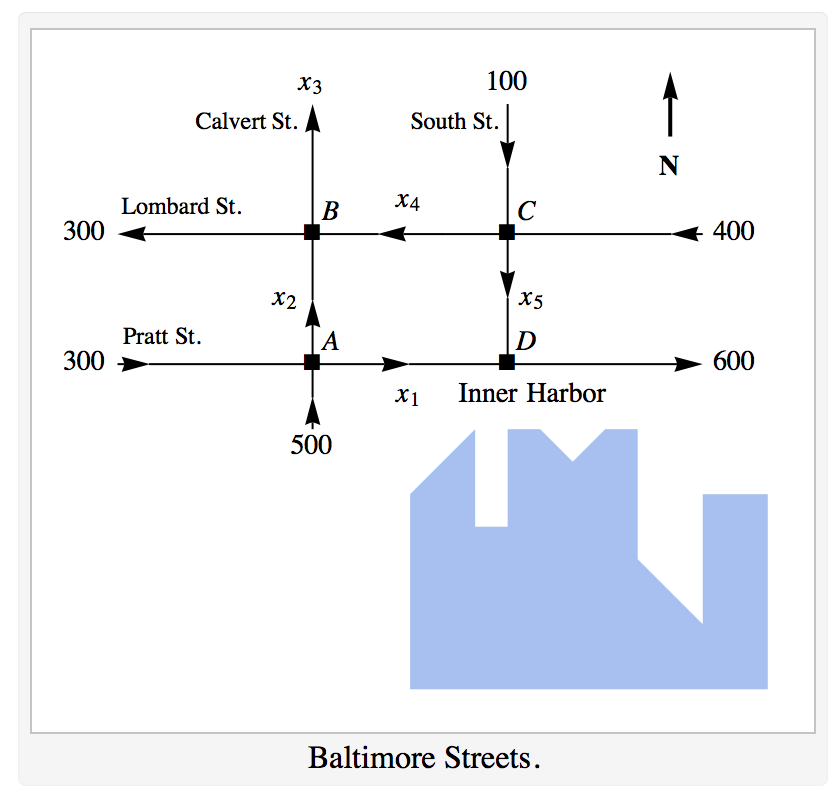
Let's solve the traffic at on the road sections: $x_1$, $x_2$, $x_3$, $x_4$ and $x_5$
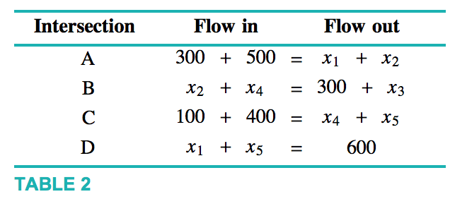
First, we need to make a table for the flows in and out of each node.
Also, the total flow into the network ($500+300+100+400$) equals the total flow out ($300 + x_3 + 600$), implying
Let's write down the system of equations
and the augmented matrix
We solve for the unknown flows using the row-reduced echelon form:
A = Matrix([[1,1,0,0,0,800],
     [0,1,-1,1,0,300],
     [0,0,0,1,1,500],
     [1,0,0,0,1,600],
    [0,0,1,0,0,400]])
print(A)
print(rre(A))
It follows that the solution is given by
Application 3: Equilibrium of a 3-sector economy (exercise 2 in Ch. 1.6)
Consider an economy with three sectors: Chemicals, Fuels, and Machinery.
- Chemicals sells 30% of its output to Fuels and 50% to Machinery, and retains the rest.
- Fuels sells 80% of its output to Chemicals and 10% to Machinery and retains the rest.
- Machinery sells 40% to Chemicals and 40% to Fuels and retains the rest.
Find the set of equilibrium prices when the price for Machinery output is 100 units.
First you must write a table for the energy flows and write out the system of equations:
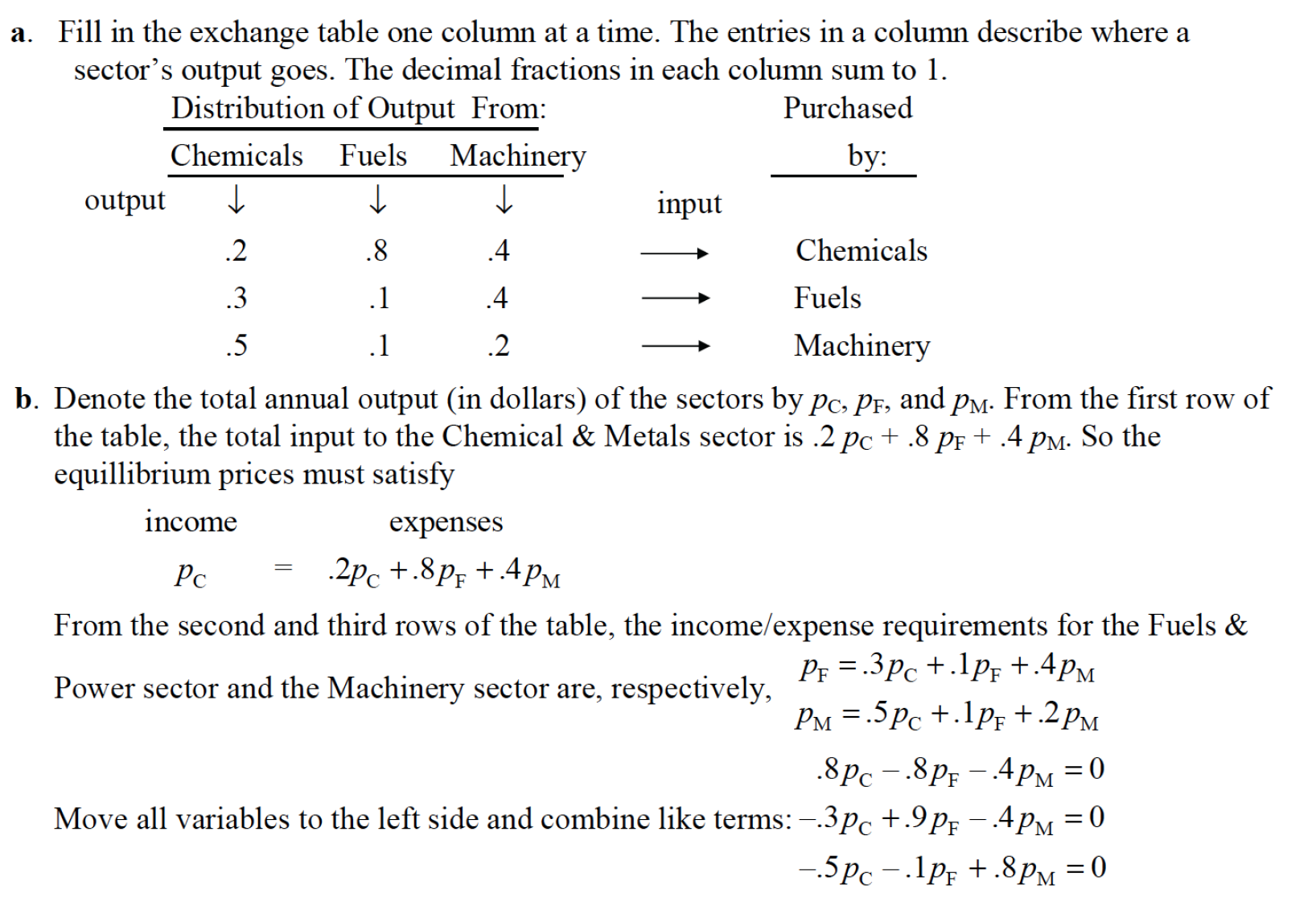
# First define the augmented matrix
a = Matrix( 10* array( [[.8,-.8,-.4,0],[-.3,.9,-.4,0],[-.5,-.1,.8,0]] ) )
a
ra = rre(a)
ra
Machine units are a free variable. If the Machine units is 12, then the Chemical units is 17 and the Fuel units is 11.